
A Short Review on Graph Neural Networks: Mechanism and Implementation
Table of Contents
Introduction
Graphical Neural Networks (GNNs) are a family of neural networks that can operate naturally on graphically structured data. They provide an effective way to do node-level, edge-level, and graph-level prediction tasks by extracting and exploiting features from the underlying graph.
This eassy wants to explain and apply graph neural networks (GNN). I have divided this report into four parts. First, we look at why we need GNNs, and some scenarios of GNN applications. Second, I explain the basic framework of GNNs from both conceptual and mathematical perspectives. Third, I will explain exactly how to train GNNs. finally, I apply a minimal GNN model to implement a node prediction task.
Learning Task & Motivation
Graph and Graph-structured Data
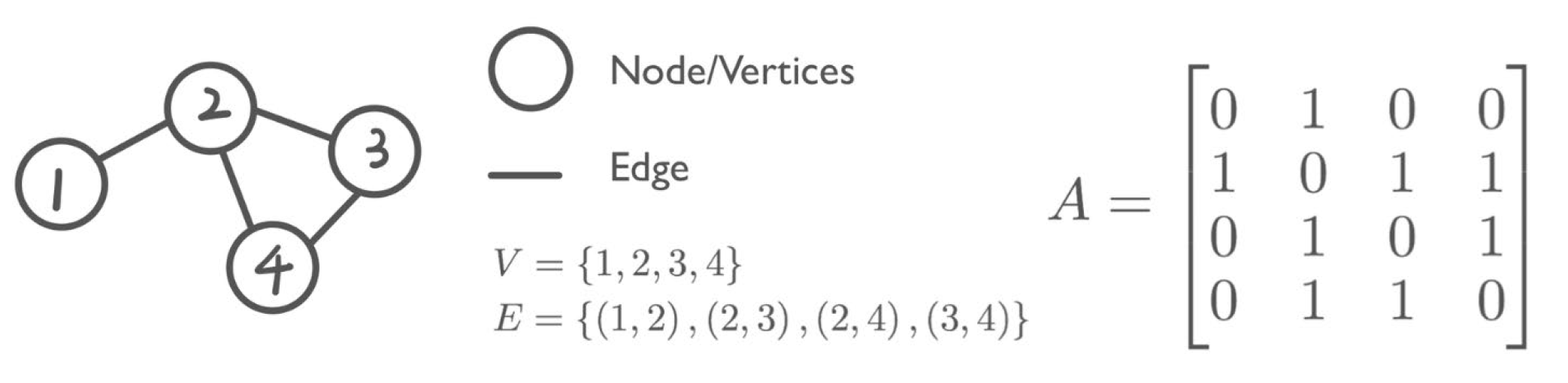
Graph-structured data is everywhere, ranging from social networks to molecules structures. A graph is a data structure consisting of two components: nodes (vertices) and edges. Formally, a graph G can be defined as \(G = (V, E)\), where V is the set of nodes, and E are the edges between them. Each edge is a pair of two vertices, and represents a connection between them.
For example (figure 1), a graph is often represented by A, an adjacency matrix. For instance, looking at a simple graph and its adjacency matrix shown below. For a graph with n nodes, A has a dimension of \((n × n)\). The adjacency matrix is a square matrix whose elements indicate whether pairs of vertices are adjacent, which means \(A_ij\) is 1 if there is a connection from node i to j, and otherwise 0. For simplicity, assume that the graph contains only undirected edges and thus \(A_ij\)= \(A_ji\). The direction and wights of edges can be added to the matrix.
Learning Tasks and Applications
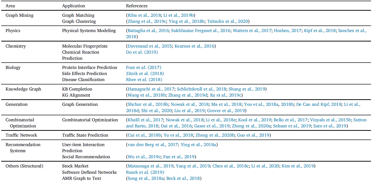
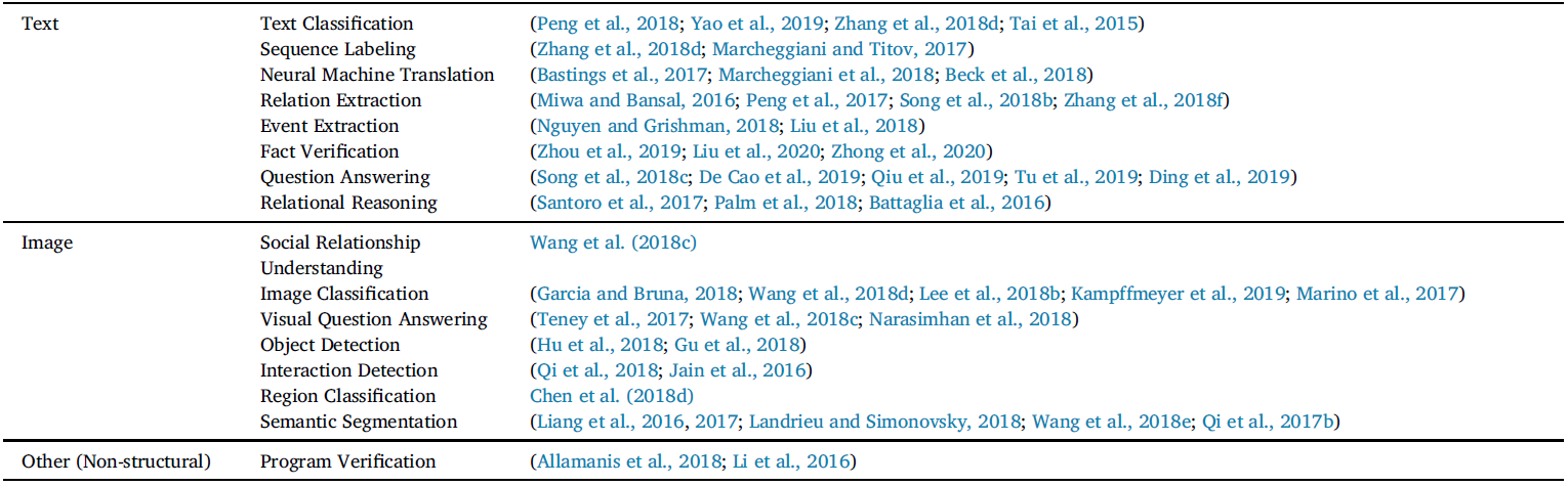
The application of machine learning on graphs spread a large range of fields with multiple learning tasks (see in Table 1).
They can be categories into three types, in node, link, and graph level respectively.
- Node classification: predict a type of a given node Typical applications include classifying users in social networks, classifying the function of proteins in the interactome (Hamilton et al., 2017) and classifying the topic of documents based on hyperlink or citation graphs (Kipf & Welling, 2016). To solve this type of learning task problem, we usually use semi-supervised training, where only part of the graph is labeled.
- Link prediction: understand graph structure and predict if two nodes are connected Recommender system is a good example, where the model is given a set of users’ reviews of different products, the task is to predict the users’ preferences and tune the recommender system to push more relevant products according to users’ interest.
- Graph classification: classify the whole graph into different categories Typical application are a wide range of industrial problems in chemistry, biomedical, physics, where the model is given a molecular structure and asked to classify the target into categories.
Why GNN
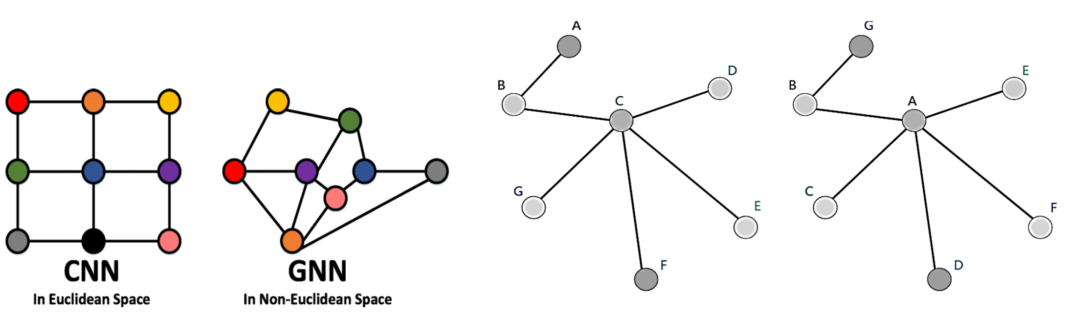
Because networks have arbitrary size and complex topological structure, which means they have no spatial locality like grids, our usual machine learning models do not apply. Convolutional neural networks (CNNs) are well-defined only over grid-structured inputs (e.g., images) in Euclidean space, while recurrent neural networks (RNNs) operate well only over sequences (e.g., text). Therefore, we need a new kind of machine learning architecture to operate on non-euclidean space, thus motivating GNN.
Also, naïve multi-layer perceptron (MLP) cannot apply to graphs either. Because networks have no fixed node ordering or reference point, any function f on graphs (adjacency matrix) should satisfy either Permutation Invariance (function does not depend on the arbitrary ordering of the rows/columns in the adjacency matrix) or Permutation Equivariance (the output of f is permuted in an consistent way when we permute the adjacency matrix). If using MLP, we flatten the adjacency matrix and feed it to a MLP, which depends on the ordering of nodes in the adjacency matrix.
Model Explanation
GNN General Framework
In this section, we will introduce the GNN formalism, which is a general framework for neural networks on graph data. Before looking at the math, we can try to intuitively understand how GNNs work.
The intuition of GNN is that it generates node embeddings, the numerical representation of nodes, by passing and aggregating neighborhood information, while ensuring the permutation invariance and equivariance. Through each layer, the embedding of each node is updated based on the aggregation of neighboring nodes, i.e., the node with only one step away. Specifically, here is the framework:
- Build multiple layers of embedding transformation
- At every layer, use the embedding at previous layer as the input
- Aggregate neighbors and self-embeddings to update the embedding
- Output the final embedding
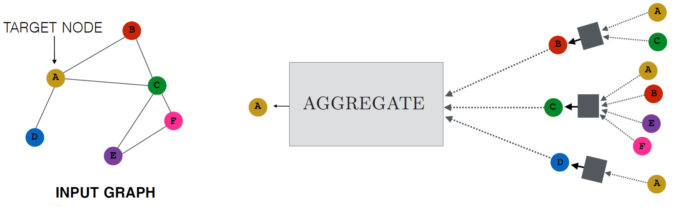
Here is the Overview of how a single node aggregates messages from its local neighborhood. The model aggregates messages from A’s local graph neighbors (i.e., B, C, and D), and in turn, the messages coming from these neighbors are based on information aggregated from their respective neighborhoods, and so on.
A single GNN Layer
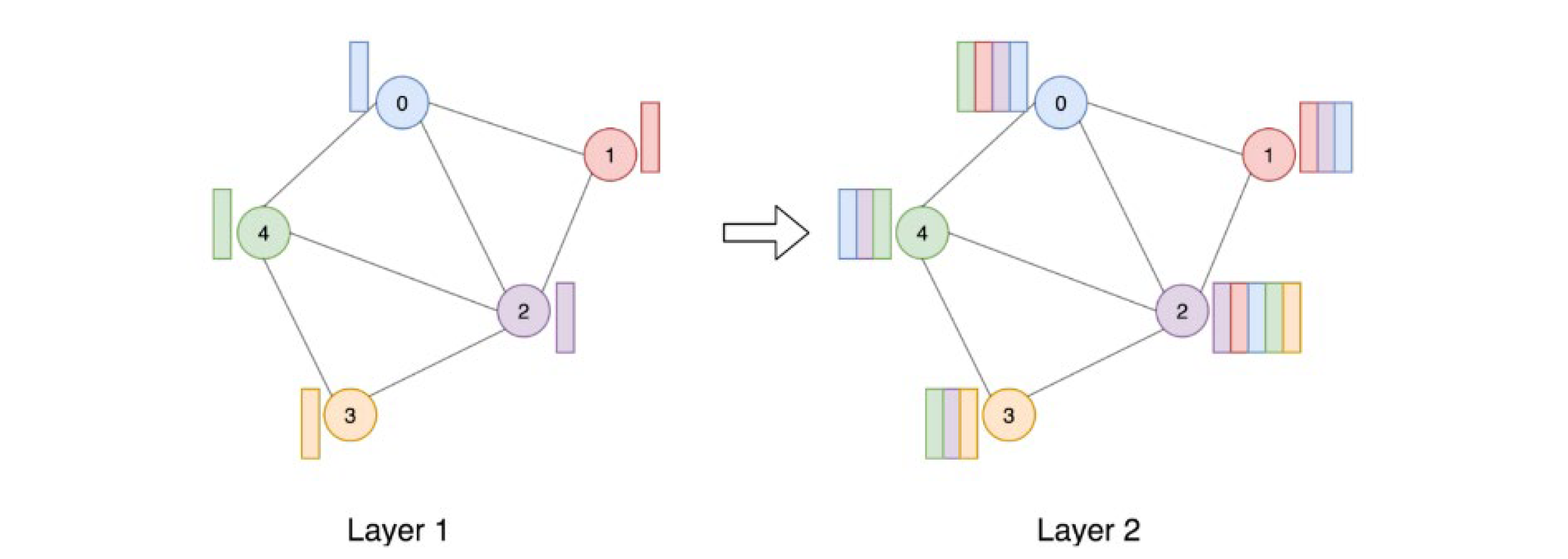
If looking at one single node, the graph above illustrates the process of node embedding updating. With respect to all nodes in the graph, the graph below shows that all node embeddings are updated in each layer (the colored rectangles beside the nodes are the node embedding vectors, and the concatenation of multiple rectangles represents the aggregation).
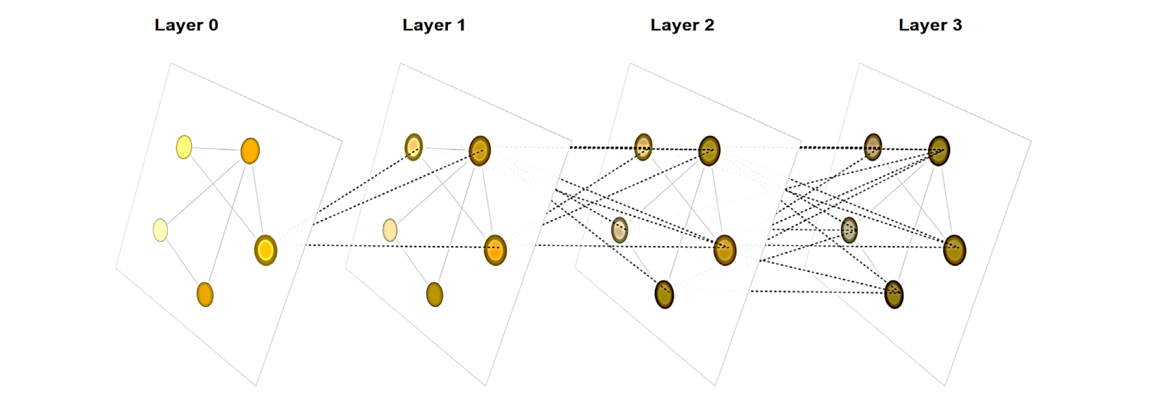
Stack Multiple GNN Layers
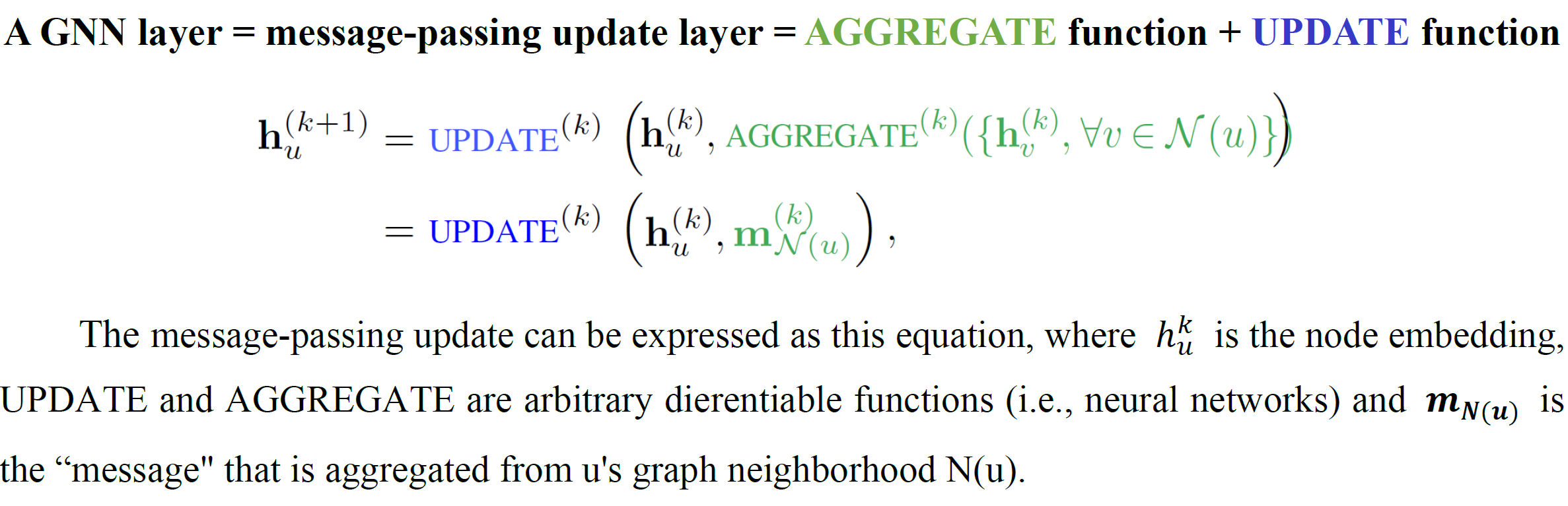
Let’s look at how multiple GNN layers are connected to form a GNN model. At each iteration k of the GNN (each layer), the AGGREGATE function takes as input the set of embeddings of the nodes in u’s graph neighborhood N(u) and generates a message m_(N(u) )^kbased on this aggregated neighborhood information.
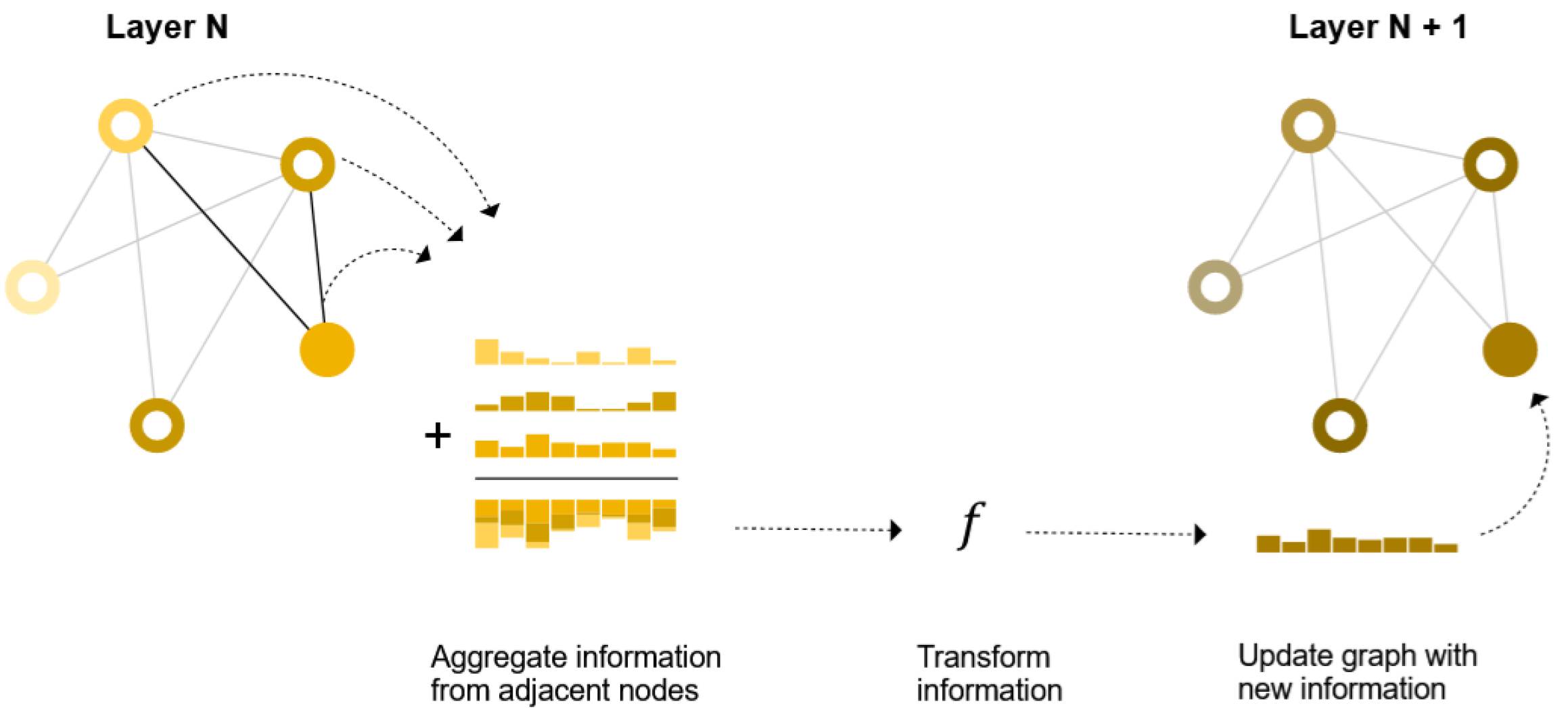
This graph shows how a node embedding is updated by accumulating information from neighbors (nodes around it) through multiple layers of a GNN. The dotted lines indicates what information are accumulated, i.e., message that is gathered and aggregated. Note that all nodes embeddings have been updated when coming to the next layer.
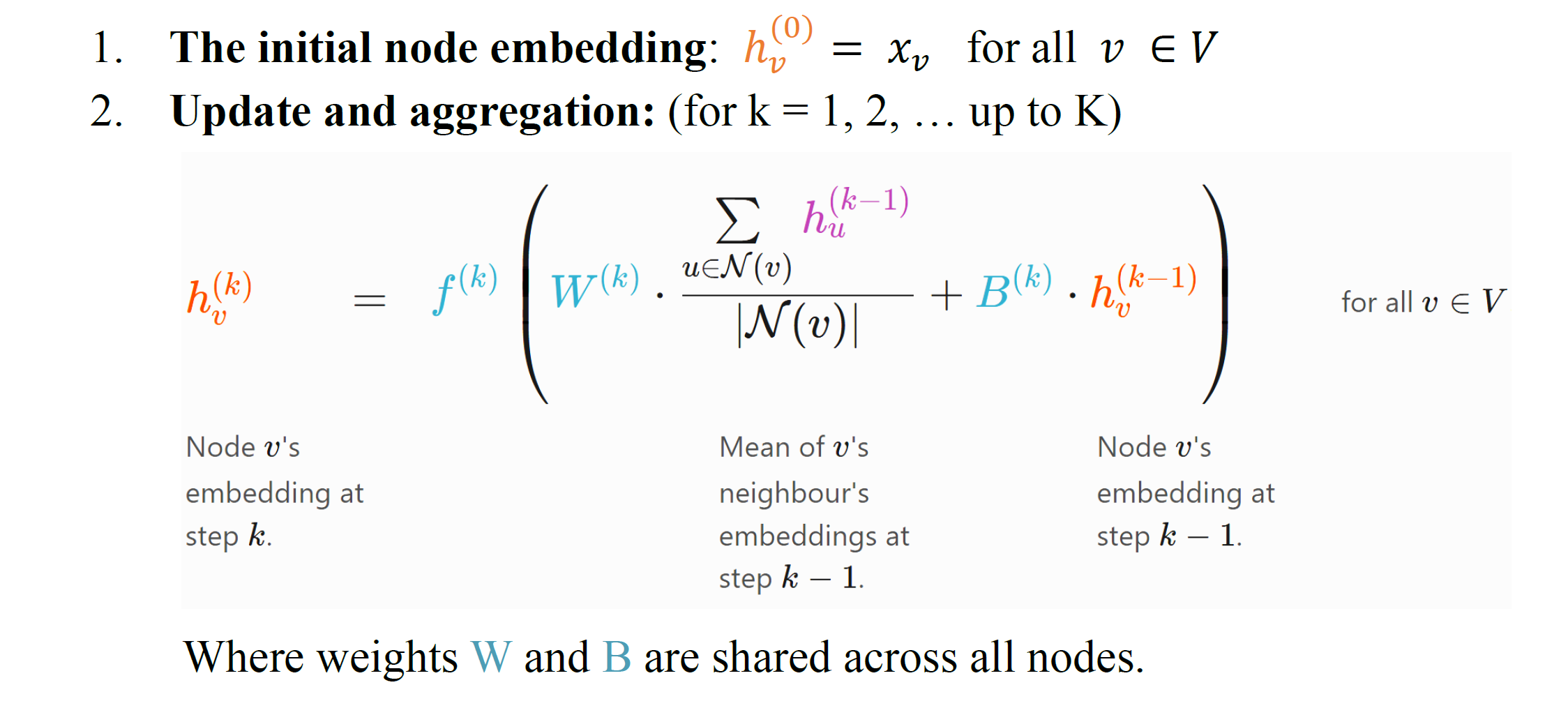
Create a Simplest GNN Layer: GCNConv
The general, abstract GNN framework is a series of message-passing iterations. In order to translate the abstract GNN framework into something we can implement, we must give concrete instantiations to the message passing functions. The most popular one is Graph Convolutional Networks (GCN). The corresponding formulation is shown below, where embedding of node v, embedding of a neighbour of node v, and learnable parameters are colored as orange, purple, and blue, respectively.
Now, let’s build the simplest GNN layer, GCNConv, which is from the “Semi-supervised Classification with Graph Convolutional Networks” paper. To implement a GCNConv layer, we just get the feature vectors of the graph and then implement the formulations provided before to compute and update embeddings.
Model Training: Learn GNN Parameters
Prediction Task: The GNN training depends on the learning task. Here we choose the semi-supervised node classification task, where we try to minimize the loss, given only some nodes in the graph are labelled.
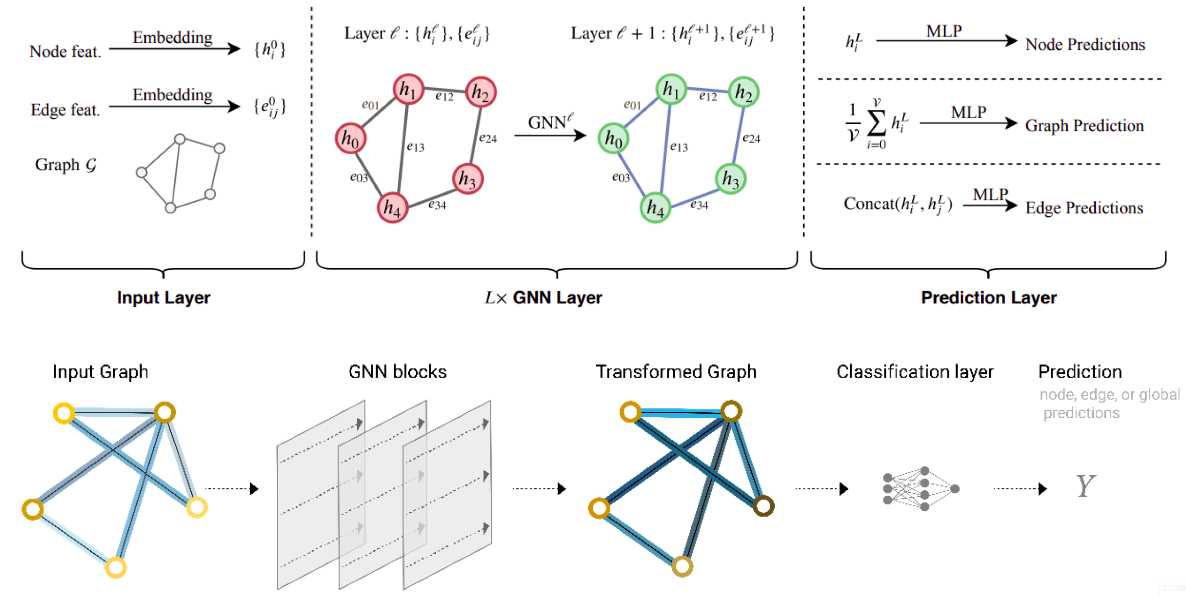
To address this problem, usually we build a end-to-end classification model, which including a GNN model to learn the node embeddings and a classifier to classify the embeddings (illustrated by figure 7). Here is the overall structure:
- Initialize node embedding
- Forward the GNN blocks
- Get final node embedding
- Apply a final classifier
Given model architecture, we now train our network parameters based on the knowledge of the community assignments. Optimization Framework: Training a GNN model is very similar to any other neural network model. We define the loss function and optimizer and then perform multiple rounds of optimization, where each round consists of a forward and backward pass to compute the gradients of our model parameters with respect to the loss derived from the forward pass. The training process follow these steps:
- Initialization: Define the model architecture, loss function, and optimizer
- Compute gradients:
- Clear gradients
- Perform a single forward pass throughout the model, taking in the initial node embeddings as the input
- Compute the loss solely based on the training nodes
- Derive gradients
- Update: Update parameters based on gradients
- Return/pint: the loss and final node embeddings
Implementation Example: Node Classification with Basic GNN Model
This example is derived from Stanford open course CS224W: Machine Learning with Graphs (Leskovec, 2021).
Dataset and Task
The learning task is a node-level prediction task, namely to classify nodes within the graph into groups. This prediction problem is analogous to image segmentation, where we are trying to label the role of each pixel in an image. I am going to apply a simplest GNN model (with three GCN layers) to first learn node embeddings and then linearly classify the nodes into four communities.
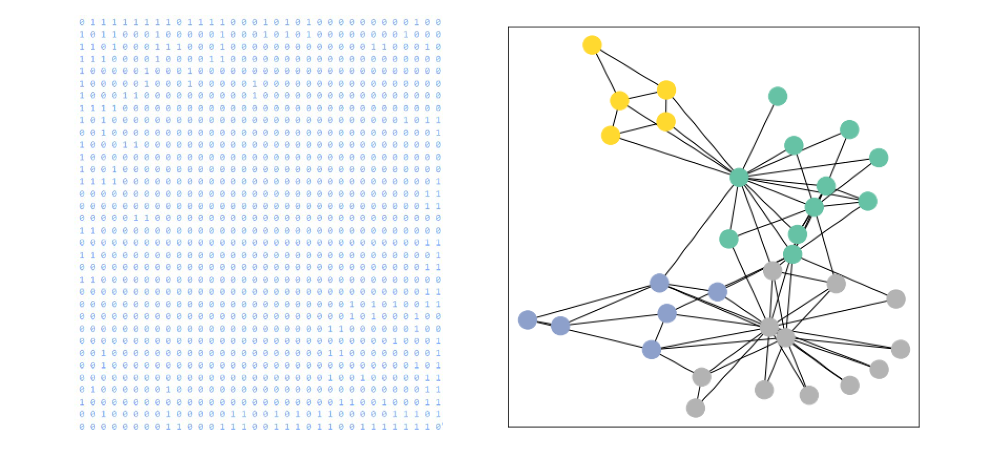
The dataset used is called Zach’s karate club, loaded from PyTorch, sourcing from the paper “An Information Flow Model for Conflict and Fission in Small Groups” (Zachary, 1977). There is only one graph in the dataset, depicting the social relationships of the members of a karate club with 34 members as nodes and the edges represent interactions between these members outside of karate. So, this graph contains 34 nodes, connected by 156 undirected, unweighted and featureless edges. Mathematically, each node in this dataset is assigned a 34-dimensional feature vector (which uniquely describes the members of the karate club). The graph is represented as an adjacency matrix (see figure 8).
Furthermore, nodes in this dataset labeled by one of four classes. These class labels are loaded from PyTorch, obtained via modularity-based clustering, following the “Semi-supervised Classification with Graph Convolutional Networks” paper, where training is based on a single labeled example per class, i.e. a total number of 4 labeled nodes. Therefore, as visualized below, the underlying graph holds 4 classes, each colored differently, which represent the community each node belongs to.
Build GNN model
As explained in the previous section, I am going to build the simplest GNN operators, the GCN layer (Kipf et al. (2017). Then, I stack three GCN layers together with a linear classifier to implement the basic GNN model. The architecture and the computation flow of this model are illustrated (aligned with the general GNN classification model).
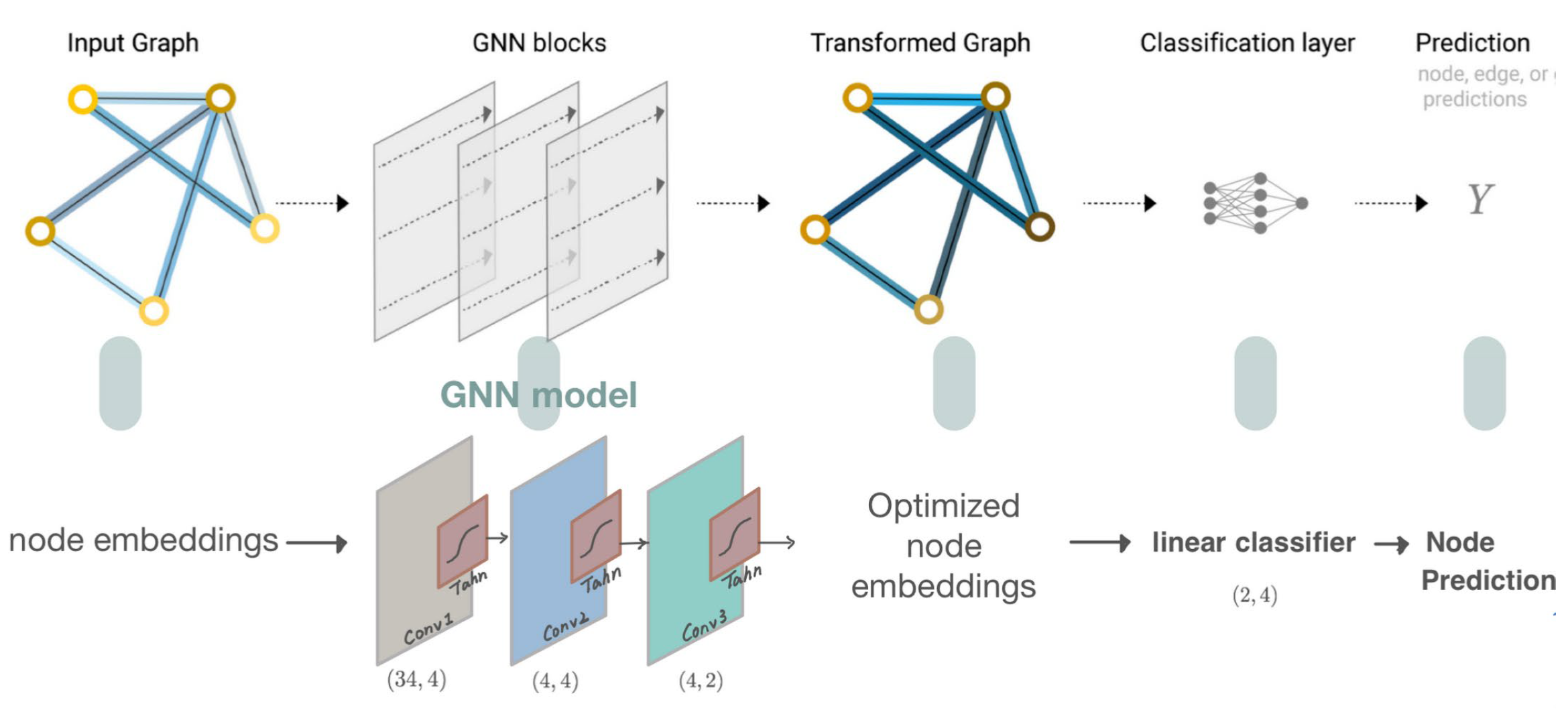
Specifically, I first define and stack three graph convolution layers, which corresponds to aggregating 3-hop neighborhood information around each node; Also, the GCNConv layers will reduce the node feature dimensionality to from 34 to 2. Each GCN layer is enhanced by a tanh non-linearity, mapping the input to between 0 and 1, which is defined as below, where x is the input element:

Finally, I add a single linear transformation that acts as a classifier to map our nodes to 1 out of the 4 classes. It return both the output of the final classifier as well as the final node embeddings produced by our GNN.
Note that before further training, the weights of our model are initialized completely at random. To enhance the model’s performance, we then train the model on the Karate Club Network by updating the network parameters based on the knowledge of the community assignments of 4 nodes in the graph (one for each community).
Training and Evaluating
Here we use semi-supervised method: We simply train against one node per class, but are allowed to make use of the complete input graph data.
To make this GNN model performs better in this dataset, I train the model following the GNN training process described previous, specifically with the following choices:
-
Loss function: cross-entropy It measures the performance of a classification model whose output is a probability value between 0 and 1. Given multiclass classification, we calculate a separate loss for each class label per observation and sum the result.
$$\mathcal{L}(y_v,\hat{y_{v}}) = -\sum_c y_{vc}\log \hat{y_{{vc}}}$$
In the semi-supervised setting, we only compute losses over labelled nodes \(\text{Lab($G$)}\) by defining a loss \(L_G\) over an input graph G as:
$$\mathcal{L}_G = \frac{\underset{v\in\text{Lab}(G)}{\sum}\mathcal{L}(y_v,\hat{y_v})}{|\text{Lab($G$)}|}$$
-
Stochastic gradient optimizer: Adaptive Moment Estimation (Adam)
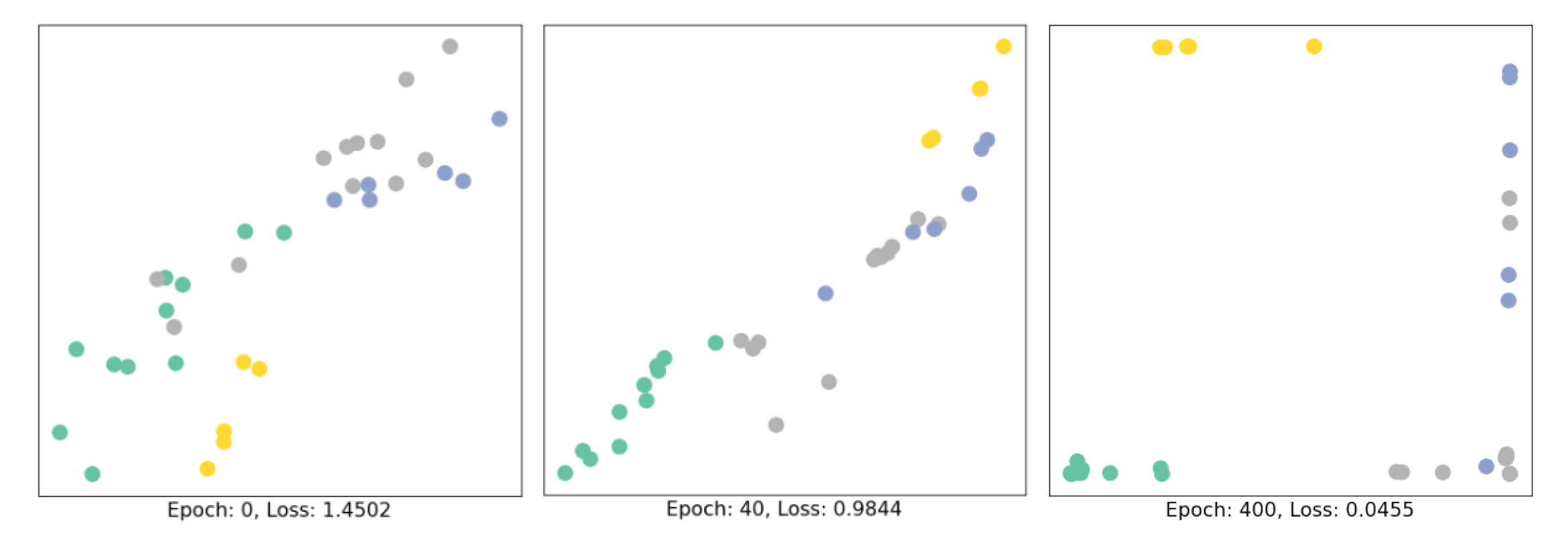
Through training, the node embeddings evolve over time. I visualize them every 10 epochs, and embeddings in the initialization (before training), 40th epoch, and 400th epoch, to give you an intuition of how they are evolved. Node belonging to different communities are separately clustered and the loss has been reduced from 1.4502 to 0.0455. The basic 3-layer GCN model seems to linearly separate the communities and classifying (most of) the nodes successfully.
References
Chaitanya Joshi, Vijay Prakash Dwivedi, Xavier Bresson. (2019). Spatial Graph ConvNets. Retrieved on September 14th, 2022, from https://graphdeeplearning.github.io/project/spatial-convnets/
Dwivedi, V. P., Joshi, C. K., Luu, A. T., Laurent, T., Bengio, Y., & Bresson, X. (2020). Benchmarking Graph Neural Networks. https://doi.org/10.48550/ARXIV.2003.00982
Hamilton, W. L., Ying, R., & Leskovec, J. (2017). Representation Learning on Graphs: Methods and Applications. https://doi.org/10.48550/ARXIV.1709.05584
Leskovec, J. (2021). CS224W: Machine Learning with Graphs [Assignment]. Stanford. http://web.stanford.edu/class/cs224w
Lin, C.-H., Lin, Y.-C., Wu, Y.-J., Chung, W.-H., & Lee, T.-S. (2021). A Survey on Deep Learning-Based Vehicular Communication Applications. Journal of Signal Processing Systems, 93(4), 369–388. https://doi.org/10.1007/s11265-020-01587-2
Sanchez-Lengeling, B., Reif, E., Pearce, A., & Wiltschko, A. (2021). A Gentle Introduction to Graph Neural Networks. Distill, 6(8), 10.23915/distill.00033. https://doi.org/10.23915/distill.00033
Scarselli, F., Gori, M., Ah Chung Tsoi, Hagenbuchner, M., & Monfardini, G. (2009). The Graph Neural Network Model. IEEE Transactions on Neural Networks, 20(1), 61–80. https://doi.org/10.1109/TNN.2008.2005605
W.L. Hamilton, R. Ying, and J. Leskovec. (2017). Inductive representation learning on large graphs. In NeurIPS, 2017.
Zachary, W. W. (1977). An information flow model for conflict and fission in small groups. Journal of Anthropological Research, 33(4), 452-473. https://doi.org/10.1086/jar.33.4.3629752
Zhou, J., Cui, G., Hu, S., Zhang, Z., Yang, C., Liu, Z., Wang, L., Li, C., & Sun, M. (2018). Graph Neural Networks: A Review of Methods and Applications. https://doi.org/10.48550/ARXIV.1812.08434