Abstract

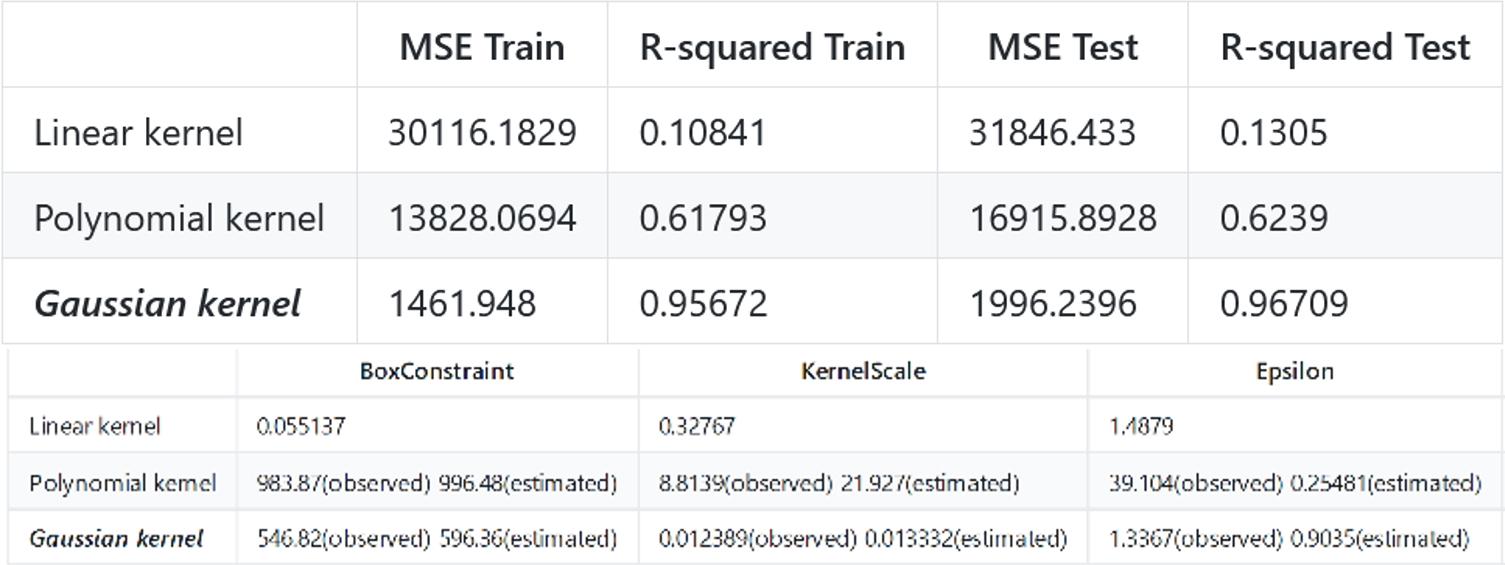
This paper adopted Supportive Vector Regression (SVR) and Least Square Regression(LSR) models to predict the traffic flow. LSR model and SVR models with linear, Gaussian, polynomial kernel separately are built and then evaluated with MSE and R-squared. The results show that the best prediction model in this case is the SVR model with Gaussian kernel (C = 546 ~ 596, Kernel Scale = 0.012 ~ 0.013, Epsilon = 0.9 ~ 1.3).

Overview

This project aims to predict traffic flow with developed SVR and LSR models, among which we can find the optimal model. The data is extracted from the dataset of traffic flow information of June 2016 collected by Highways-England.

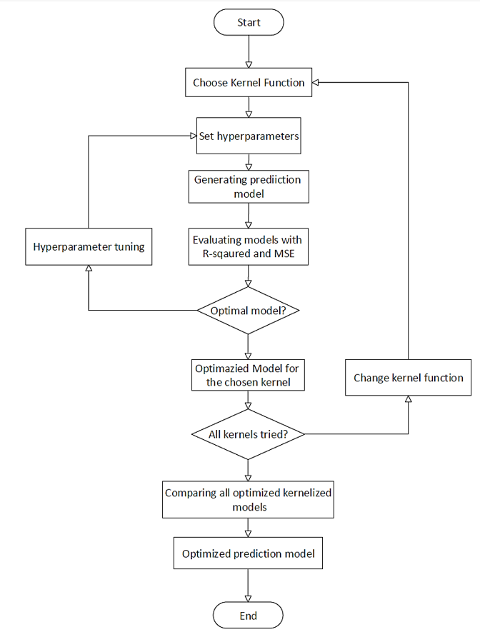
Matlab is used to implement the prediction modeling. In order to find the optimized model with each type of kernel (linear, polynomial, Gaussian), corresponding hyper-parameters are tuned according to the performance. Models’ performance is measured with MSE and R-squared.

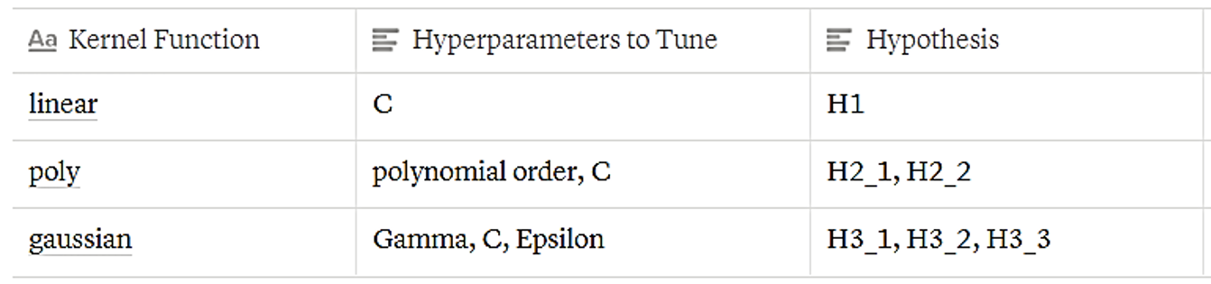
I followed the principle of controlling variables when tuning the hyperparameters of SVR models. That is, I not only test three cases for each kernel, but a series of cases with one parameter changed and others hold constant. This tuning strategy enables me to see the influence power and relations of hyper-parameters. Specifically, I test six hypotheses, each of which focus on a certain parameter.

The findings show that the SVR model performs the best, with Gaussian kernel (C = 546 ~ 596, Kernel Scale = 0.012 ~ 0.013, Epsilon = 0.9 ~ 1.3) among all models. Also, kernel function is the most important factor for accuracy. Additionally, the results shed light on the relations among parameters.

This paper will be organized into three main sections, besides the introduction and references: (1) mathematical formulation and Implementation, (2) experimental results, and (3) results discussion.

Detailed experiments and calculations are still updating… (to this page)

Discussion

The influential factors, as described before, are the kernel functions and corresponding hyperparameters. I will explain the influence power of each of them and their relationships in detail. In short, learning from the hypothesis testing and the optimization modeling, we come to the following conclusions.

LSR VS. SVR

SVR model does not always perform better than the LSR model, whose kernel function chosen contributes to the differences. But still, we can see the best function in SVR exceeds the performance of LSR best model, which means that if we choose kernel and parameters carefully, SVR may generally have better performance than LSR.

Comparing Kernel Functions

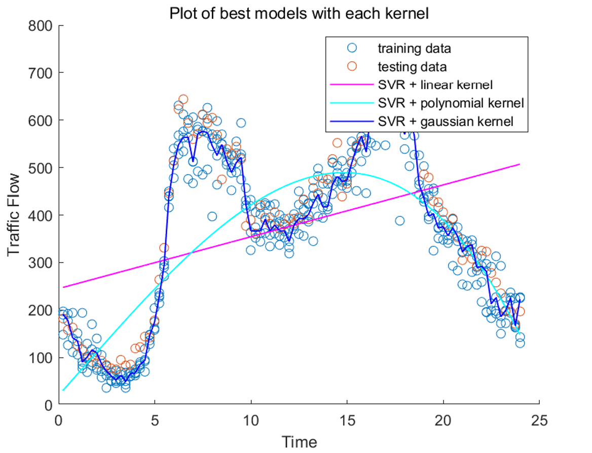
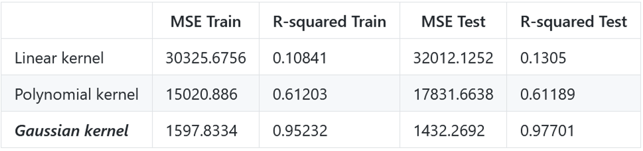
First we compared models. Obviously Gaussian kernel works the best in this case. Unsurprisingly the linearly kernelized SVR model performs the poorest, since the traffic flow data is curved, i.e. nonlinear.

Though we obtained the optimized model of linear kernel (test R-squared: 0.108, train R-squared: 0.130) and polynomial kernel (test R-squared: 0.618, train R-squared: 0.624), they still perform worse than less optimized Gaussian kernel (test and train R-squared ranges from 0.82 to 0.97). This result indicates that kernel function is very influential to the model’s precision, overweighting the hyperparameters.

Why the Gaussian kernel works so well? We may find in figure 3 that polynomial kernel model is too smooth and linear kernel model is too straight.

Hyper-parameters

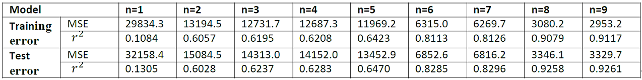
Then we look into the hyperparameters. As shown in the graphs and tables, the optimized model is highlighted in bold and italic. In the following part of this section, I will interpret and discuss these results, grouped by kernel type.

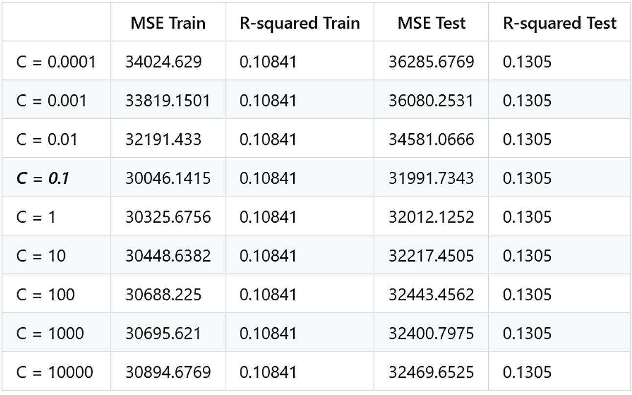
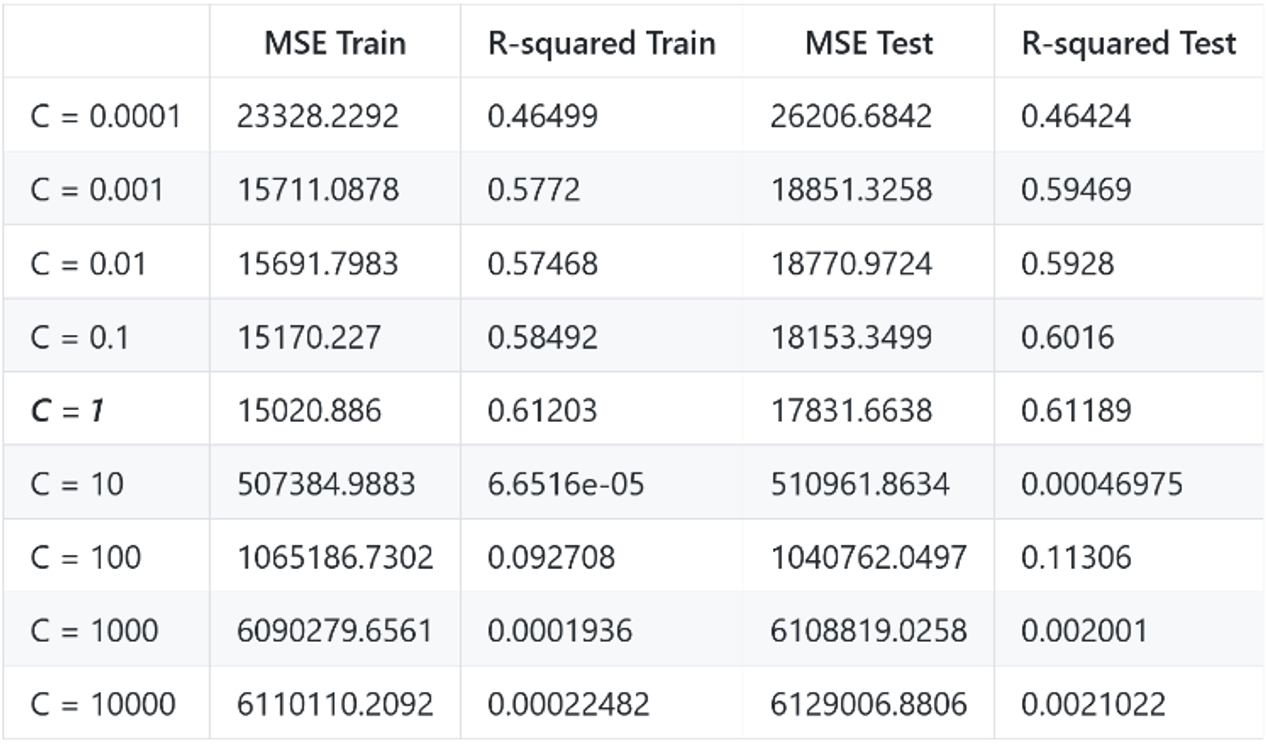
For the Linear kernel, the real optimized model (auto-found by Matlab) occurs when C = 0.055137.

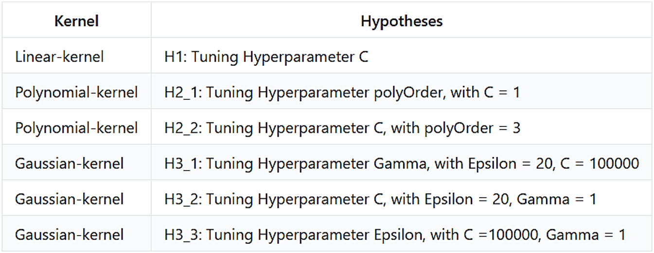
H1: The optimized model is obtained with C = 0.1, since it has the minimal training and testing MSE. It is closer to the real optimized function.

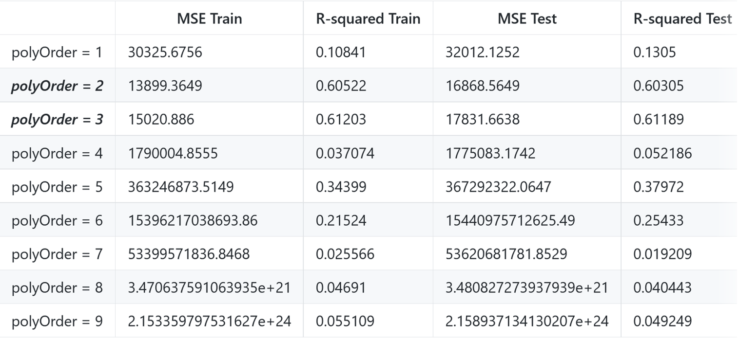
We can see that linear kernel is mainly impacted by the box constraint. I’ve tried to change other parameters but they do not affect the model a lot. For the Polynomial kernel, the real optimized model (auto-found by Matlab) occurs when C = 996 ~ 983.
H2.1: The optimized model is obtained with polyOrder =2 or 3, if C is 1.
H2.2: The optimized model is obtained with C =1 with the polynomial order set to 3.

This value is very different from the really optimized C, which might because of the polyOrder set different from the overall real optimized model’s.

Accidentally, the two cases validate each other because they find the same optimized model, with polyOrder = 2 or 3, and C as 1. However, because C is too small, we cannot obtain the real optimized model.

For the Gaussian kernel, the real optimized model (auto-found by Matlab) occurs when C = 546 ~ 596, Kernel Scale = 0.012 ~ 0.013, Epsilon = 0.9 ~ 1.3.

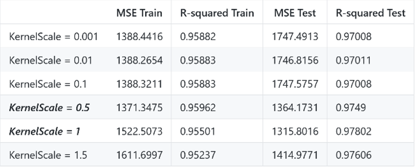
H3.1: The optimized model is obtained with Kernel Scale = 0.5 or 1, holding Epsilon = 20, C = 100000.
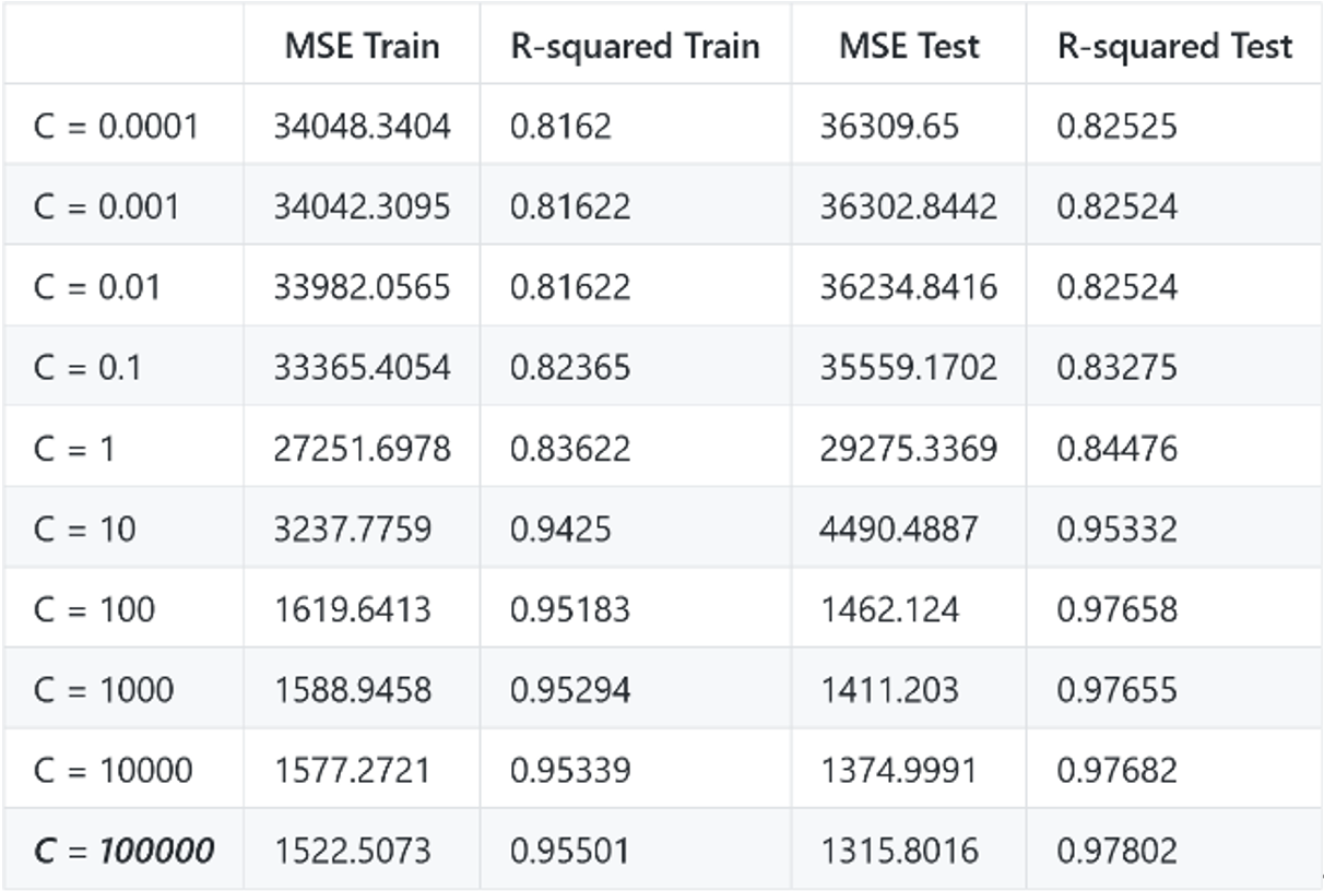
H3.2: The optimized model is obtained with C = 100,000, with Epsilon = 20, Gamma = 1.
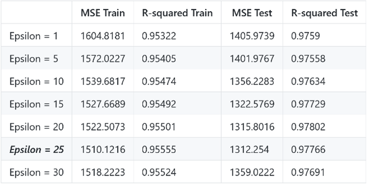
H3.3: The optimized model is obtained with Epsilon = 25, holding C = 100000, Gamma = 1.

From the results of Gaussian kernel, we can see how the three parameters influence each other. That is, the value of a certain parameter will not always be the optimized, if other parameters are set differently. Only considering all of them can we find the overall optimization of the model.

What’s more I assume that a large C works so well because our test and training data are very similar, thus preventing the problem of overfitting which always occurs when C is very huge. I set C up to 100,000 in H3_2, but the train and test MSE are low; and train and test R-squared (0.955, 0.978) are very high.

In conclusion, besides the optimized models, we also have several interesting, additional findings.

The most important factor of model prediction accuracy is the choice of kernel function.
For the linear kernel, C matters the most.
For the Gaussian kernel, a large C works well because of the similarity of test and training data.
For the gaussian kernel, three hyper-parameters are closely related.

Limitations

Though intuitively I get some thoughts about the hyper- parameters’ impacts and their relations, the order in which they should be tuned and the complexity (running time, memory occupation) are still unclear or left out of consideration. Besides, the test cases are still biased and are not in a huge amount.

We need further examination of the nature of parameters and kernel functions.

Possible Improvements

We should not rely on the auto optimization function em- bedded in the Matlab. Instead, we can choose algorithms to implement optimization manually, in which way we can get a deeper insight of the model and the parameters’ influence.

Specifically, the following tuning strategies can be leveraged.

The first is cross-validation. It uses different portions of the data to test and train a model on different iterations.
Another approach is grid search. That is, using a grid of parameter settings, with step size decreases.
Additionally, the running time and memory usage should be taken into consideration. For example, we can monitor the time cost when testing models. Also, think of more effective searching algorithm and examine the features of the dataset more closely.

Project Highlight

In the project, I firstly built three cases with different hyper-parameter settings for each kernel type. However, I soon realized that three cases are far from adequate for us to draw any meaningful conclusions. Especially, for Gaussian kernel, which has three editable parameters, carefully change each parameter while keeping other parameters constant is necessary. Therefore, I tried much more cases for each kernel with controlled parameters unchanged and tested six hypotheses to see the impact power of each hyper-parameter.

References

[1] “Fit a support vector machine regression model - MATLAB fitrsvm.” https://www.mathworks.com/help/stats/fitrsvm.html (accessed Oct. 20, 2020).

[2] Platt, John, Sequential Minimal Optimization: A Fast Algorithm for Training Support Vector Machines, 1998.

[3] S. Boyd and L. Vandenberghe, Introduction to applied linear algebra: Vectors, matrices, and least squares. Cambridge: Cambridge University Press, 2019.

[4] Numerical Methods for Engineers. New York: McGraw-Hill, 2015.

Project | Optimize Supportive Vector Machine and Least Square Regression Models for Traffic Flow Prediction

Table of Contents