
Project | Does Economic Development Promote Gender Equality? Analysis with Road Traffic Mortality as the Instrumental Variable
Table of Contents
1. Introduction
Gender equality has been paid much attention. It was set as a main objective in World Development Report 2006: Equity and Development, and promoting gender equality becomes progressively more crucial in enhancing economic dynamics, life standards, and combating poverty (Marone, 2016). Yermoshenko (2016) goes on to argue that among all aspects, gender equality in education is especially important, and Sustainable Development Goals (SDGs) focus on quality education and reducing gender inequality.
As gender equality, especially equality in educational opportunity, is closely associated with economic development, we are interested in the following questions. Does economic development causally affect gender equality in education? If it does, to what extent does it promotes or inhibits gender equality in education? An increasing number of research study the causal relationships between them, and most of them use regression analysis based on cross-countries data (Kabeer & Natali, 2013). However, the causality is not easy to identify and interpret due to a potential bias. It could be the case that gender equality in education contributes a lot to the economies’ development, and thus the results show that countries with higher economic development tend to have less gender inequality in education.
This bias, in econometrics, is attributed to the endogeneity caused by simultaneity, which means dependent and independent variables are codetermined. Therefore, this paper uses instrumental variable analysis to address this problem of endogeneity. This approach begins with the choice of instrumental variable, a factor that is highly correlated with the instrumented variable, namely the endogenous regressor, and not indirectly correlated with other influential factors or directly affects the dependent variable. Then the exogenous part of the explanatory variable will be isolated and predicted by the regression with the instrumental variable included. Thus, as the endogenous variable is instrumented, we could interpret the causal effect based on the regression model.
This paper aims to answer the question that whether economic development exerts a causal effect on gender equality in education and how much the effect might be. The regression analysis and instrumental variable analysis are adopted. In the regression model, the gender gap in adult literacy rates is set as the dependent variable, representing gender equality in education; gross national income (GNI) per capital is set as the explanatory variable, representing the economic development. Considering the bias originating from simultaneity, I choose the number of road traffic mortality per 100,0000 people as the instrumental variable for GNI per capita. This instrument is strongly correlated with GNI per capita and satisfies the other two conditions of instrumental variable. The data is separately drawn from the dataset collected by UNESCO Institute for Statistics, World Bank, and OECD. The results report that GNI per capita has a statistically significant causal effect on the gender gap in adult literacy rates, proving support for the assumption that economic development promotes gender equality in education.
The paper is organized as follows. The second section describes the data analyzed, including the sources, treatment, and summaries. The second section discusses the robustness of choosing road traffic mortality as the institutional variable for GNI per capita. The forth section provides economic and econometric models. The fifth section presents the estimates results, discussion, and limitation, followed by the sixth section of the conclusion.
2. Data
2.1 Dataset
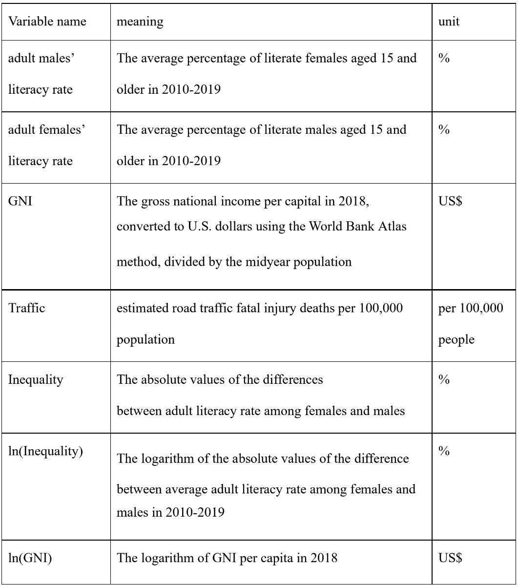
The analysis requires information on gender inequality in education, economic development, and road traffic mortality. Both gender inequality and economic development need to be measured properly. Thus, I choose the data of gender gap in adult literacy rates and GNI per capita to represent these two kinds of information, respectively. I find the data separately since there is currently no dataset contain all the data needed, and the names, meanings and units of the variables analyzed are presented in Table 1.
Gender Gap in Adults’ Literacy Rates. Though this data is not directly provided, I find the adults male and female literacy rates in UNESCO Institute for Statistics, where adults are persons aged 15 and older. I calculate the gender gap by subtracting the adult females’ literacy rates from the adult males’ literacy rates of given countries and then taking the absolute values of them. Furthermore, to represent the gender inequality in educational opportunity which should reflect a relatively long-term situation, I choose the average values of literate rates among adults in 2010-2019, instead of the values in a particular year. Accordingly, this variable is named as Inequality which means the absolute values of the differences between adult literacy rate among females and males, measured with percentage.
GNI Per Capita. It is the gross national income (GNI) of economies in 2018. To simplify the expression, I renamed it just as GNI in the regression analysis. The data is found from World Bank national accounts data, and OECD National Accounts data files. It is converted to U.S. dollars using the World Bank Atlas method, divided by the midyear population. GNI is the sum of value added by all resident producers plus any product taxes not included in the valuation of output plus net receipts of primary income from abroad. Though calculated in national currency, it is usually converted to U.S. dollars at official exchange rates for comparisons across economies. The world Bank also adopts the Atlas method of conversion in order to smooth fluctuations in prices and exchange rates. It applies a conversion factor that averages the exchange rate for a given year and the two preceding years, adjusted for differences in rates of inflation between the country. From 2001, these countries include the Euro area, Japan, the United Kingdom, and the United States.
Road Traffic Mortality. This variable simply renamed as Traffic, is found in World Health Organization’s Global Status Report on Road Safety 2018 through Global Health Observatory data repository. Considering the population differences among countries, I choose the relative number of road traffic mortality to population, namely road traffic mortality per 100,000 people.
2.2 Data Summary
All the data are collected from countries and economics around the world. Originally there are 226 economies in the dataset, including countries and larger regional cross-country economies like South Asia. However, I exclude 12 cross-country economies since I would like to analyze the data of countries around the world. Hence, there are totally 214 countries in the dataset, and in the following analyses, missing values are eliminated.
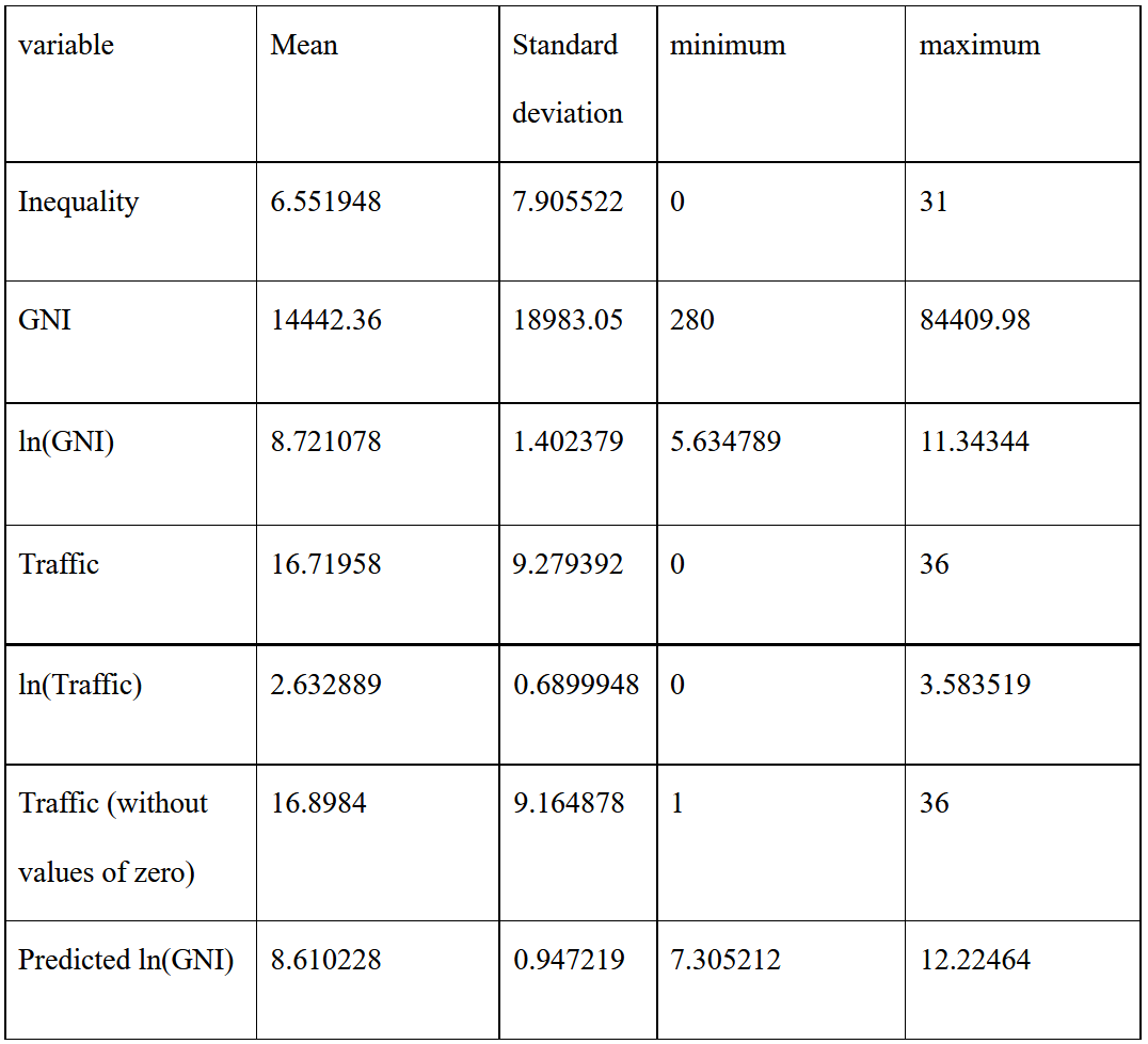
In this section I would summarize the data and check if the datasets are well cleaned, namely whether there are some mistakes. Also, the outliers that provide no meaningful information are taken into consideration. furthermore, the treatment of the data is detailed. The summaries of the data before and after treated are shown in Table 3.
Gender Gap in Adults’ Literacy Rates. This variable contains 154 observations, with an average value of approximately 6.55% and a standard deviation of about 7.91%. It might look a little strange that in 13 countries, such as Botswana, Qatar, and Uruguay, the adult males’ literacy rate is less than that among adult females because in common sense, females generally have fewer education opportunities than males have. However, such a situation could happen, and the data of these countries is very likely not a mistake. Hence, I take the absolute values of them and analyze them as other data since I aim to examine gender inequality, no matter which gender seems to be in the advantage.
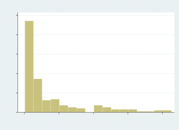
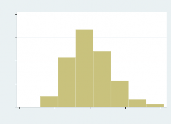
GNI Per Capita. This variable has 191 observations, with 14442.36 dollars on average. Its standard deviation approaches 18983.05 dollars that is large and reflect the possibly large variation in the data, and the distribution of it is highly skewed to the right (Figure 1). Thus, re-expression might be needed later. There are some very large values of GNI per capita that need to be checked. After carefully checking, I choose to consider them not problematic. These countries include highly developed countries like The United States with 63,080 dollars GNI per capita and countries that are rich but have quite small populations, such as Iceland, Norway, and Switzerland. So they seem to not be mistaken. But I would consider to re-express them later since these outliers are, indeed, quite influential to the results.
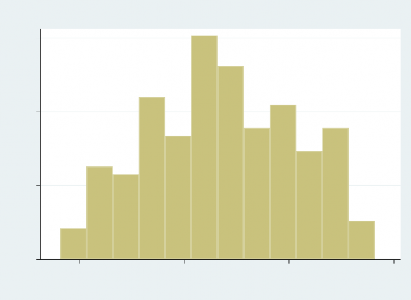
Due to the large standard deviation, skewness and some influential data with high values, I re-express GNI per capita by taking the logarithm of it, named as ln(GNI). I use logarithm safely because the values of GNI per capita in the dataset are positive. The distribution of the logarithm of GNI per capita is given in Figure 2, which is much more normally distributed than the formal one. Also, after taking the logarithm of GNI per capita, the standard deviation of 1.402379 dollars is much smaller and the outliers with very high values are less influential because the differences between their values and other values are much smaller, and thus they need not to be eliminated.
Road Traffic Mortality. Its sample size reaches 189. The special values are equal to 0, which might be mistaken. But after further examining the values, I found they possibly are not mistakes. Their values could be approximately zero if the number is too small since, after all, the unit is per 100,000 people, One of the countries with zero road traffic mortality is Monaco, whose population of 2018 is only 38,682 which is much less than 100,0000. Similarly, another country is San Marino with only a population of 33,562. Therefore, the values of zero could be possibly not mistakes. But indeed, they are very special.
For better future analysis, I then take the logarithm of road traffic mortality. Though the logarithm automatically excludes the two values of zero, it is fine because these two data exert little impact on the results. As shown in the fifth and seventh row in Table 3, the mean is changed by about 0.6% which is very small. Also, as analyzed before, they are quite special and could be discussed separately.
3 Robustness of Road Traffic Mortality as the Instrumental Variable
3.1 GNI Per Capita as an Endogenous Regressor
In the regression model, only when the explanatory variable is exogenous can we claim the causal effects that the change in the independent variable leads to the change in the dependent variable. Therefore, GNI per capita needs to be exogenous, which means it is unrelated to the other factors affecting gender equality in education. One main source of endogeneity is simultaneity, which means two variables are codetermined. In this case, simultaneity is said to occur if GNI per capita affects the gender gap in adult literacy rates and at the same time be affected by it. Thus, the model cannot support a causal interpretation. Unfortunately, the simultaneity seems to be true.
Many researchers examine the role played by gender equality in the economic development process. A review of the literature shows that gender equality, particularly in education, has a consistent and robust contribution to economic growth (Kabeer & Natali, 2013). Perrin (2015) believes that gender equality was a key trigger for the transition where economies move out of a long period of stagnation into a state of sustainable economic growth. Meanwhile, Kazandjian, Kolovich, Kochhar, and Newiak (2019) find that gender inequality does harm to the economic growth by reducing the diversity of economies, in particular in low-income and developing countries. This might because gender gaps in educational opportunity constrain the human capital available in an economy (Kazandjian et al., 2019). Accordingly, the problem of simultaneity is very likely to exist and thus GNI per capita suffers from endogeneity.
3.2 The Correlation between Road Traffic Mortality and GNI Per Capita
There is a reasonable theoretical motivation for using road traffic mortality as the instrumental variable for GNI per capita. Economic development is find associated with road traffic mortality, especially in countries with accelerated economic growth. For example, with rapid economic growth in the last decade, Vietnam suffers from increasing road traffic injuries which becomes one of the leading causes of death (Nagata et al., 2011). The same situation was faced by Iraq before 2013, where the economic growth was accompanied by the increase in the number of vehicles as well as road traffic injuries (Al Saad & Sondorp, 2013). Similarly, Al-Reesi et al. (2013) analyze that economic growth in Oman is related to an increase in motorization rates, which has a direct relationship with increased road traffic mortality.
3.3 Check the Conditions for Instrumental Variable
For a variable to be used as the instrumental variable (IV), the following three assumptions need to be satisfied: (1) it should be highly correlated with the endogenous variable; (2) it should be uncorrelated with the regression error term, which represents the other factor affecting the dependent variable; and (3) it should be related to the outcome only through its association with treatment, which means it has no direct or indirect effect on the independent variable. It turns out that road traffic mortality meets these three conditions, which are discussed in detail as follows.
3.3.1. High Correlation with the Endogenous Variable
The first condition requires a high correlation between the instrumental variable and the endogenous variable. Road traffic mortality is closely associated with GNI per capita, which is demonstrated by the correlation, scatterplot, and the regression results, satisfying the first condition. Also, the strength of the instrumental variable is measured. The instrumental variable should not be included if it is weak since it will be underpowered to detect the effect even with a large sample size.
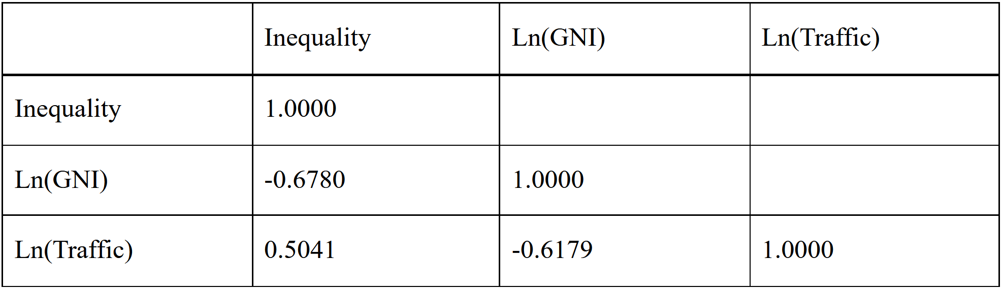
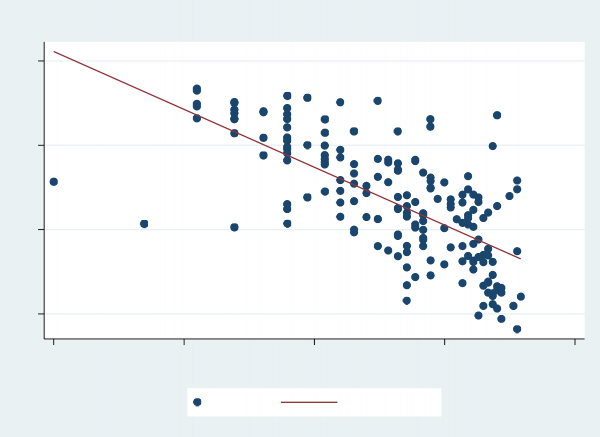
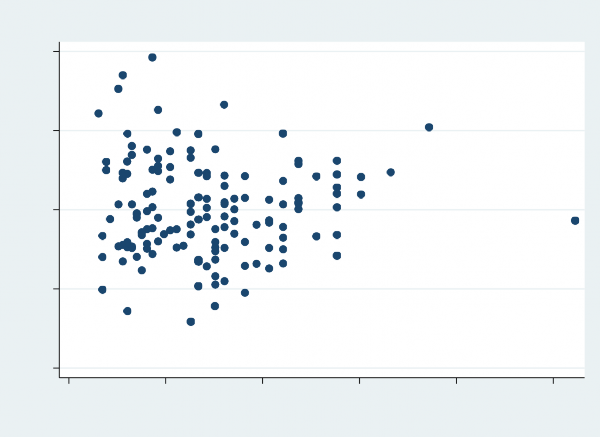
As shown in Table 3, the correlation between the logarithm of road traffic mortality per 100,0000 people and the logarithm of GNI per capita of a given country between is - 0.6179, which is sufficiently large. Also, as we can see in Figure 3, it shows a very strong, negative linear trend, which indicates a high correlation.
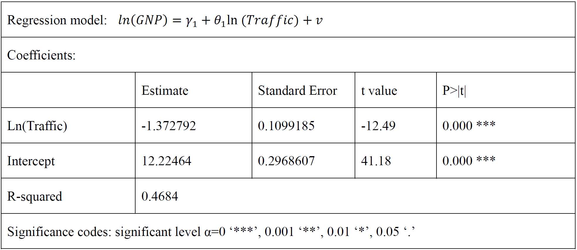
Then I run the first-stage regression in 2SLS (Equation 1), with the logarithm of road traffic mortality per 100,0000 people as the explanatory variable and the logarithm of GNI per capita of a given country as the dependent variable.

The results are reported in Table 4. With a relatively large R-squared, the logarithm of road traffic mortality per 100,0000 people prove to be, indeed, strongly correlated with the dependent variable. R-squared of 0.4684 is also large, which means 46.84% of the variance of the logarithm of GNI per capita can be explained by the addition of the logarithm of road traffic mortality per 100,0000 people to the model.
Moreover, the strength of this instrument is reflected by the t-statistic for 𝐻0:𝜃1=0 which is the hypothesis that the logarithm of road traffic mortality per 100,0000 people has no effects on GNI per capita of a given country. When using 2SLS estimator and single instruments, the absolute value of t-statistic less than 3 is considered potentially problematic. By contrast, the t-statistic reported as -12.49 is much greater than 3, showing that this instrumental variable is sufficiently strong.
3.3.2 Exogeneity
The second condition emphasizes the exogeneity of the instrumental variable. One potential problem with using road traffic mortality as the instrumental variable is that road traffic injury may be related to the educational situations within the country. Nevertheless, I would show that though the road traffic mortality might be affected by the population’s education level, it does not meaningfully bias the estimates.
Nagata (2011) claims that the leading causes of road traffic injury include alcohol consumption, poor awareness of traffic safety, and violation of traffic laws. For example, Suphanchaimat, Sornsrivichai, Limwattananon, and Thammawijaya (2019) find that in Thailand, one-third of the affected riders had drunk alcohol before the ride, and the helmet law was enforced poorly that only 43.7% riders use helmets. Furthermore, Thomas et al. (2013) conclude that more than half of traffic injuries are human-caused. These human causes, indeed, can be affected by the education level of the population. Well-educated people, in general, are more likely to observe the traffic regulations and have better safety awareness. Thus, the traffic environment in countries with a high education level of the population might be better than those with a low education level, generating less road traffic mortality. The educational situation could be partly reflected by adult literacy rates.
However, in this paper I choose the gender gap in literate rates, not simply the absolute values of overall literate rates. The gender gap cannot effectively reflect the general education level, and vice versa. Though the overall literacy rates are possibly quite influential on road traffic injuries, it is less likely that road traffic mortality is strongly influenced by the gender differences in literacy rates in education.
3.3.3 No Direct Effect on the Dependent Variable
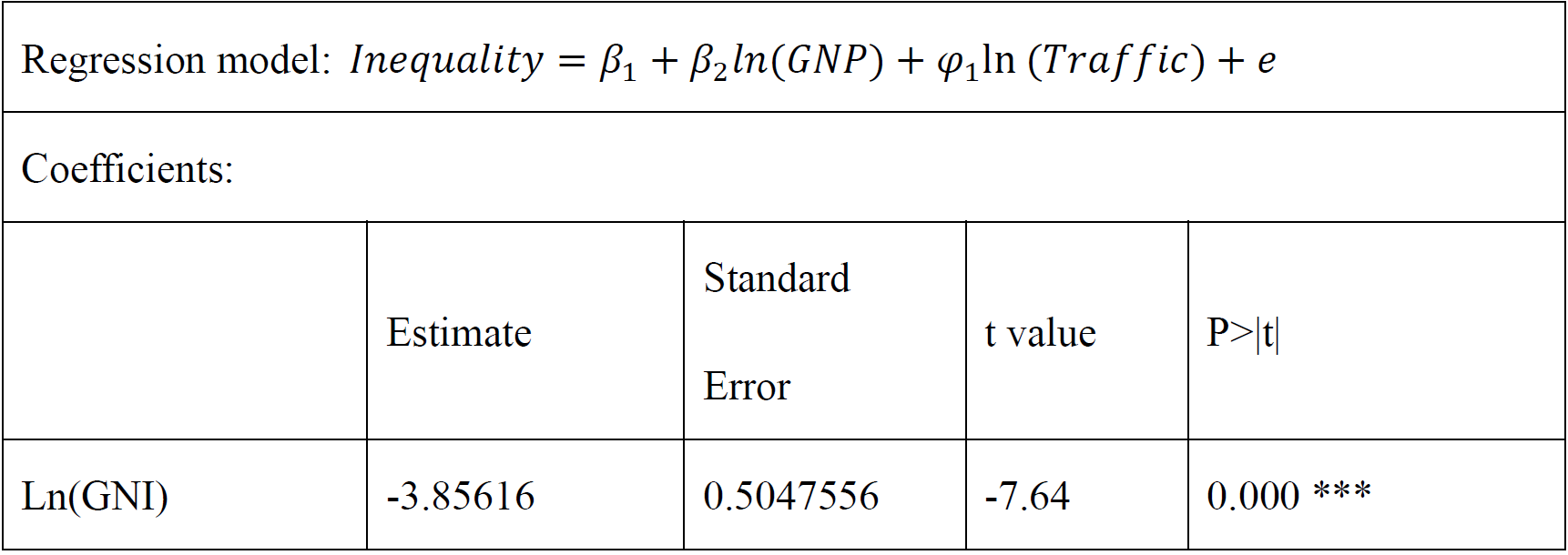
To meet the third condition, road traffic mortality, set as the instrumental variable, should not affect the gender gap in adult literacy rates directly. First of all, in common sense, it is not very likely that road traffic mortality has a direct effect on the gender gap in adult literacy rates. I will further prove it by building and testing a regression model where the dependent variable is the gender gap in adult literacy rates and the explanatory variables include GNI per capita and road traffic mortality. If road traffic mortality, indeed, has no direct effect on gender inequality in educational opportunity, it should not belong to Equation (2) as an explanatory variable, thus ensuring that the only effect of road traffic mortality on the gender gap in adult literacy rates is through economic development represented by GNI per capita.
In other words, if testing the model, we should fail to reject the hypothesis that road traffic mortality exerts no effect on the gender gap in adult literacy rates.

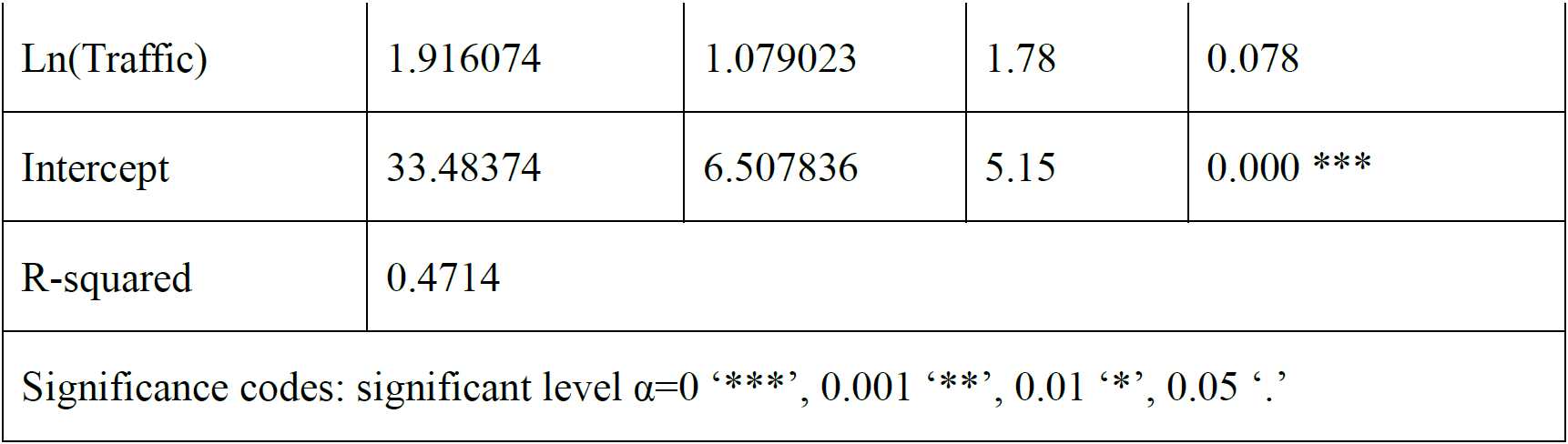
Table 5 reports the results of the regression estimates. The P-value of the estimated coefficient of the logarithm of road traffic mortality reaches 0.078, which is larger than 0.05. It means that the coefficient for the instrumental variable road traffic mortality is not statistically significant at a 5% significance level. Thus, we fail to reject the null hypothesis that the coefficient equals zero and conclude that there is no evidence to show road traffic mortality has a direct effect on the gender gap in adult literacy rates.
4. Model
4.1 Economic Model
According to the analysis in the introduction, the second and the third section, many research results show that there are close associations between gender inequality in education and economic development, and this paper aims to find the causal effect between them.
Hence, I choose gender gap in adult literacy rates to represent the gender inequality in education and GNI per capita to represent the economic development. These two variables are built into the economic model as the dependent variable and the explanatory variable respectively. Furthermore, to determine whether the effect of GNI per capita on the gender gap in adult literacy rates exists and how much it is, the econometric model is built.
4.2 Econometric Model
This paper interests in estimating the parameters of the following regression where 𝛽1is an intercept parameter, 𝛽2 is a slope parameter representing the effects of GNI on gender inequality in education, and e is the error term.

Then I go on to build the Two-Stage Least Squares (2SLS) regression model, including the first-stage regression and the second-stage regression. In the first-stage regression (1), 𝛾1is an intercept parameter, 𝜃1is a slope parameter, ad v is an error term.

To build the second-stage regression, I estimate the first-stage equation by OLS and obtain the fitted value (4). Then I replace the endogenous variable ln(GNI) in the original simple regression model to obtain the second-stage regression (Equation 5), where 𝛽𝛽1is an intercept parameter, 𝛽2is the Two-Stage Least Squares Estimator, ad e is an error term

5. Results and Discussion
5.1 Estimates
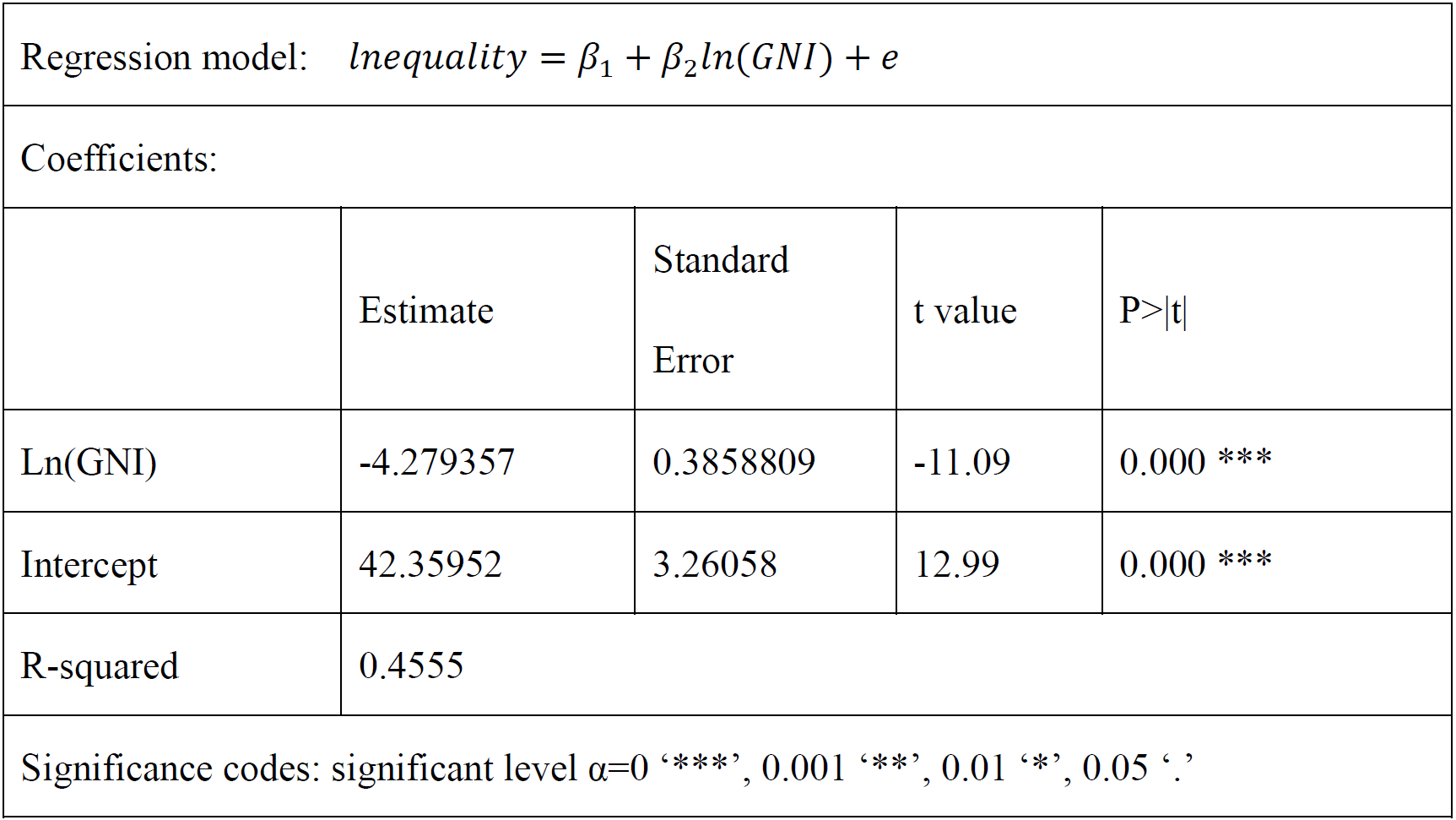
OLS. The estimates of the models, output by Stata 16, are as follows. Table 6 reports OLS estimates of Equation (3), where the dependent variable is the gender gap in adult literacy rates and the explanatory variable is the logarithm of GNI per capita. The estimated effect is that a one percent increase in GNI per capita will lead to an approximately 0.0428% decrease in the gender gap in adult literacy rates. Considering the difference unites, the results seem to be realistic. The regression has a R-squared of 0.4555, meaning that 45.55% of the variance in the gender gap in adult literacy rates can be accounted for by the logarithm of GNI per capita. With P-value approaching zero, we reject the hypothesis that GNI per capita exerts no effect on the gender inequality reflected by different adult literacy rates. The estimates suggest a significant relationship between the logarithm of GNI per capita of a given country and the gender gap in adult literacy rates, which allows the further 2SLS estimate with instrumental variable. This is because the fitness of the regression model with instrument would be less than the original regression without instrument.
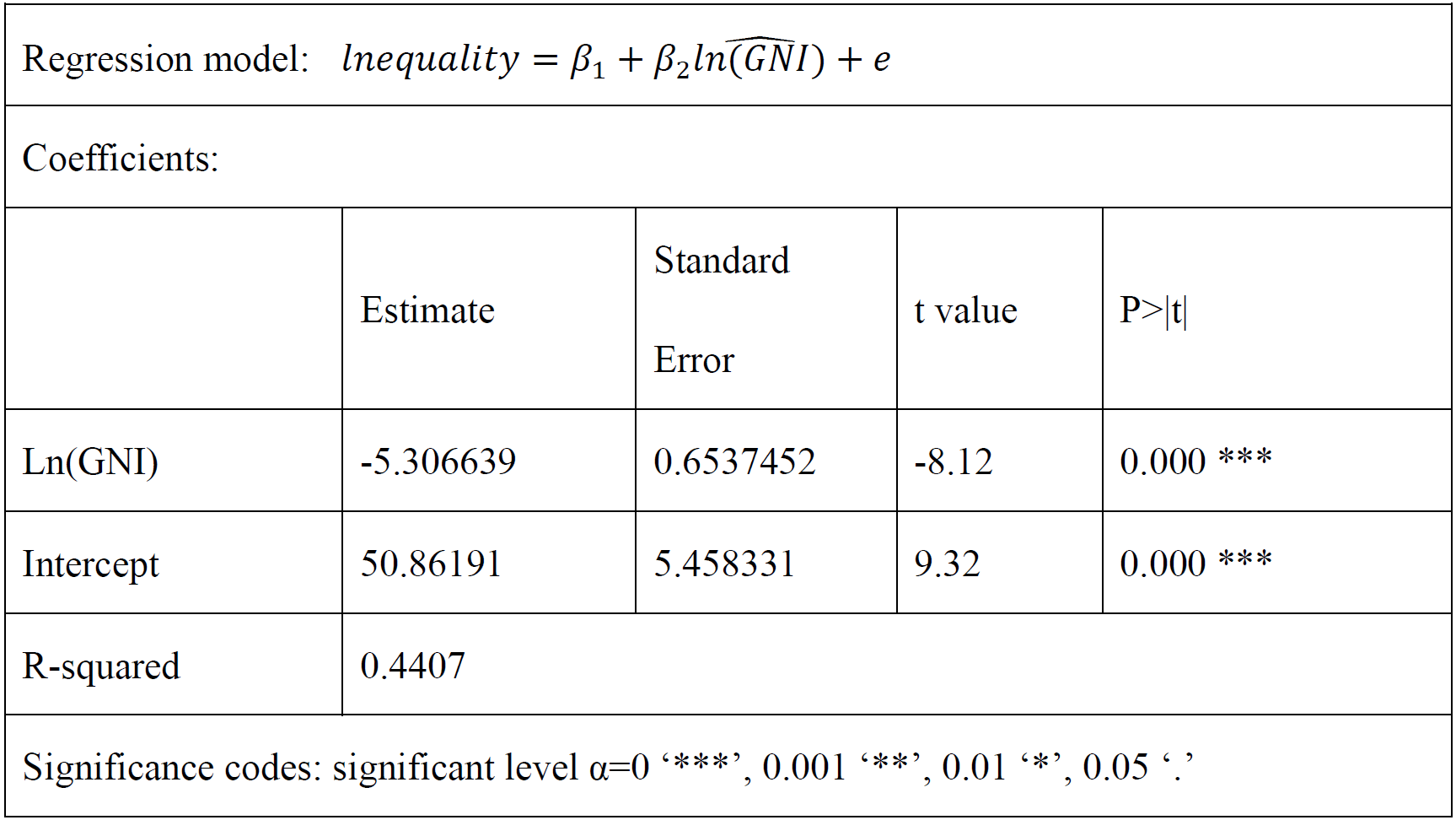
2SLS Second-Stage Regression. Table 7 reports the estimates of Equation (5), the second-stage regression, which is also what I will build conclusions from. In this regression, the explanatory variable is the value of the logarithm of GNI per capita predicted by Equation (1), and the dependent variable is the gender gap in adult literacy rates, the same one as in the original regression model without the use of instrument. The coefficient of the predicted value of the logarithm of GNI per capita is estimated to be -5.306639, indicating that a one percent increase in the predicted GNI per capita gives rise to a decrease in the gender gap in adult literacy rates of about 0.0531%. Though the estimated values of effect seem to be small, we should consider the difference in units and find that it might be realistic. The R-squared generated by this regression is 0.4407, suggesting that the predicted value of the logarithm of GNI per capita could explain 44.07% variance in the gender difference in adult literacy rates. Moreover, the absolute values of the t-statistics for two coefficient estimates are both larger than 8, providing P-values approaching zero. Thus, I reject the null hypothesis that the logarithm of GNI per capita should not be included in the regression and the intercept should be zero. Shortly speaking, according to the results, we could see a a significant relationship between the gender gap in adult literacy rates and predicted GNI per capita with instrument of road traffic mortality.
In the original regression, Equation (3), we fail to interpret the effect of GNI per capita on gender gap in literacy rates as causal because the GNI per capita, as discussed in the third section, is an endogenous regressor. But after using road traffic mortality as the instrumental variable, the effects of changes in GNI per capita alone are isolated. In other words, the endogenous part of GNI per capita that are correlated with other influential factors is separated and the exogenous part of it is left in the second-stage regression, namely Equation (5). Therefore, based on the second-stage regression, we could interpret a causal effect of GNI per capita on the gender gap in adult literacy rates. That is to say, one percent increase in GNI per capita results in about 0.053% decrease in the gap between adult literacy rates among males and females. Hence, economic development contributes to gender equality in educational opportunity.
5.2 Re-check the Robustness of the model
I will check the robustness of the model by assessing the goodness-of-fit of the regression and judging if the instrumental variable is needed based on the estimated difference caused by the inclusion of it.
Goodness-of-Fit. As shown in Table 7, the R-squared is 0.4407 that is relatively large in single regression models. It means that 44.07% of the variance in the gender gap in adult literacy rates can be accounted for by the logarithm of GNI per capita with instrument of the logarithm of road traffic mortality. Also, both the coefficient estimates of the intercept and the explanatory variable are statistically significant with a significant level less than 0.1%.
Moreover, the distribution of the residuals of the second-stage regression model (Figure 4) is roughly normal though it is slightly skewed to the right, and the scatterplot (Figure 5) shows no interesting patterns. The summary of the residuals shows that the mean value is 0.0825208% which is very close to zero. Accordingly, the traits of the residuals demonstrate that the second-stage regression model seems to fit well to a certain degree.
Instrumental Variable. The robustness of choosing road traffic mortality as the instrumental variable is shown in the second section, and it is further proved by the difference between the OLS and 2SLS estimates. The estimates of the coefficient of the logarithm of GNI per capita is -4.279357 in the original OLS regression without the instrument and - 5.306639 in the 2SLS regression with the instrument. The difference in values between them is about 1.03, which is a change of 21% that is large. It means that GNI per capita, indeed, is an endogenous regressor and thus the use of instrumental variable road traffic mortality is needed.
5.3 Extensions and Limitations
Admittedly, the findings should be viewed in light of several limitations. The primary limitation to the generalization of these results is the certain existence of omitted variables. The simple regression model with only one explanatory variable can hardly present the real situations fully. Though the R squared of 0.4407 is quite large among single regression models, undeniably only 44.07% variance in the gender difference in adult literacy rates could be explained by this model. But I do not expect this simple regression model to explain all influential factors on gender inequality in education, and instead, I am only interested in interpreting the causal effect of GNI per capita on the gender gap in literacy rate. This limitation does not indicate a fatal flaw in this paper since the main purpose has been achieved. Further study could add more regressors in the model, which helps to estimate the effects of GNI on gender equality in education more preciously.
Also, the research findings of this study were limited by the different characteristics of the relationships between economic and road traffic mortality in different levels of development. Blumenberg et al. (2018) find that countries with predicted gross domestic product (GDP) per capita values above or below the median experience different kinds of changes in road traffic mortality. For countries with higher GDP, the recent years have seen a statistically significant reduction trend on the road traffic mortality rates, while for those with lower GDP, there is a significant positive trend of their road traffic mortality rates. Similarly, many researchers identify a nonlinear relationship between road traffic mortality and economic development (Suphanchaimat, 2019). Accordingly, future research could try to get better use of road traffic mortality as the instrumental variable by examining the situations in developed and developing countries separately. Also, different stages in development of a given country generate different results. Thus, a good choice is to explore the relationships between economic growth rate and road traffic mortality.
Conclusion
This paper examines the causal effect of economic development on gender equality in education by using regression analysis. In the regressions, the dependent variable is the gender difference in adult literacy rates and GNI per capita of a given country is the explanatory variable. To give a causal interpretation, the regressor should be exogenous, which means it is not correlated with other factors that might affect the dependent variable. However, the explanatory variable, GNI per capita, proves to be endogenous. Therefore, the instrumental variable analysis is adopted, where road traffic mortality per 100,0000 people is the instrumental variable for GNI per capita.
The main finding is that a one percent increase in GNI per capita is estimated to lead to about 0.053% decrease in the gap between adult literacy rates among males and females. The R-squared of the regression model with GNI per capita instrumented by road traffic mortality is 0.4407, which means 44.07% of the variance in the gender gap in adult literacy rates can be accounted for by the model. Moreover, the coefficient estimates are statistically significant with a significant level less than 0.1%. In short, the estimated results are, to some extent, reliable. Thus, I conclude from the results that economic development improves gender equality in educational opportunity of a given country. In addition, as argued by Kabeer and Natali (2013), though economic development does contribute to the gender equality in education, there is no guarantee that the economic growth alone could resolve the critical problem of exiting gender inequality. Therefore, progressive strategies need to be reformulated and adopted to keep fighting against gender inequality in any aspect with any form.
References
Al-Reesi, H., Ganguly, S. S., Al-Adawi, S., Laflamme, L., Hasselberg, M., & Al-Maniri, A. (2013). Economic growth, motorization, and road traffic injuries in the sultanate of oman, 1985-2009. Traffic Injury Prevention, 14(3), 322-328. doi:10.1080/15389588.2012.694088
Al Saad, N. A., & Sondorp, E. (2013). Road traffic injuries in iraq. Lancet, the, 381(9879), 1720-1720. doi:10.1016/S0140-6736(13)61079-X
Blumenberg, C., Martins, R. C., Calu Costa, J., & Ricardo, L. I. C. (2018). Is brazil going to achieve the road traffic deaths target? an analysis about the sustainable development goals. Injury Prevention, 24(4), 250-255. doi:10.1136/injuryprev-2017-042473
Ferreira, F. H., & Walton, M. (Eds.). (2005). World development report 2006: Equity and development (Vol. 28). World Bank Publications.
Kabeer, N., & Natali, L. (2013). Gender equality and economic growth: Is there a Win‐Win? IDS Working Papers, 2013(417), 1-58. doi:10.1111/j.2040-0209.2013.00417.x
Kazandjian, R., Kolovich, L., Kochhar, K., & Newiak, M. (2019). Gender equality and economic diversification. Social Sciences, 8(4) doi:http://dx.doi.org/10.3390/socsci8040118
Marone, H. (2016). Demographic dividends, gender equality, and economic growth: The case of cabo verde. IMF Working Papers, 16(169), 1. doi:10.5089/9781475524246.001
Nagata, T., Takamori, A., Kimura, Y., Kimura, A., Hashizume, M., & Nakahara, S. (2011). Trauma center accessibility for road traffic injuries in hanoi, vietnam. Journal of Trauma Management & Outcomes, 5(1), 11-11. doi:10.1186/1752-2897-5-11
Perrin, F. (2015). An exploration of the cliometric relationship between gender equality and economic growth 1. Economics and Business Review, 1(1), 34. doi:10.18559/ebr.2015.1.4
Suphanchaimat, R., Sornsrivichai, V., Limwattananon, S., & Thammawijaya, P. (2019). Economic development and road traffic injuries and fatalities in thailand: An application of spatial panel data analysis, 2012–2016. BMC Public Health, 19(1), 1-15. doi:10.1186/s12889-019-7809-7
Thomas, P., Morris, A., Talbot, R., & Fagerlind, H. (2013). Identifying the causes of road crashes in europe. Annals of Advances in Automotive Medicine. Association for the Advancement of Automotive Medicine. Annual Scientific Conference, 57, 13-22.
Yermoshenko, A. (2016). Insuring progressive approach to gender equality in education: the Swedish approach. University Economic Bulletin, 1(30), 159-162. Retrieved from https://economic-bulletin.com/index.php/journal/article/view/347